Embedded Motion Control 2013 Group 1: Difference between revisions
m (→Line detection) |
|||
| Line 132: | Line 132: | ||
|- | |- | ||
| B | | B | ||
| | | [[#Lines|Lines.msg]] | ||
| pico_line_detector | | pico_line_detector | ||
| /pico/line_detector/lines | | /pico/line_detector/lines | ||
| Line 139: | Line 139: | ||
|- | |- | ||
| C | | C | ||
| | | [[#Localization|Localization.msg]] | ||
| pico_situation | | pico_situation | ||
| /pico/situation/localization | | /pico/situation/localization | ||
| Line 146: | Line 146: | ||
|- | |- | ||
| D | | D | ||
| | | [[#Situation|Situation.msg]] | ||
| pico_situation | | pico_situation | ||
| /pico/situation/situation | | /pico/situation/situation | ||
| Line 153: | Line 153: | ||
|- | |- | ||
| F | | F | ||
| | | | ||
| | | | ||
| | | | ||
| Line 160: | Line 160: | ||
|- | |- | ||
| G | | G | ||
| | | | ||
| | | | ||
| | | | ||
| Line 166: | Line 166: | ||
| | | | ||
|} | |} | ||
==== Pico standard messages ==== | |||
To let the different [http://wiki.ros.org/Nodes nodes] communicate with each other they send [http://wiki.ros.org/Messages messages] to each other. ROS defines already a number of different messages such as the [http://wiki.ros.org/std_msgs standard] and [http://wiki.ros.org/common_msgs common] messages. The first provides a interface for sending standard C++ datatypes such as a integer, float, double, et cetera, the latter defines a set of messages which are widely used by many other ROS packages such as the [http://docs.ros.org/api/sensor_msgs/html/msg/LaserScan.html laser scan] message. To let our nodes communicate with each other we defined a series of messages for ourself. | |||
===== Line ===== | |||
The line message includes two points, p1 and p2, which are defined by the [http://wiki.ros.org/geometry_msgs geometry] messages package. A point can have x-, y- and z-coordinates we however only use the x- and y-coordinate. | |||
geometry_msgs/Point32 p1 | |||
geometry_msgs/Point32 p2 | |||
===== Lines ===== | |||
The lines message is just a array of the Line.msg. Using this messages we can send a array of lines to another node. | |||
Line[] lines | |||
===== Localization ===== | |||
The localization message includes 4 [http://docs.ros.org/api/std_msgs/html/msg/Float32.html float32]'s. Angle holds the angular mismatch of the robot with respect to the wall. The distance_front holds the distance with respect to the front wall if any is detected, in case no front wall is detected a special value is assigned. Respectively distance_left and distance_right are used for the distance w.r.t. wall for the left and right side. | |||
float32 angle | |||
float32 distance_front | |||
float32 distance_left | |||
float32 distance_right | |||
===== Reasoning ===== | |||
===== Situation exit ===== | |||
The situation exit message uses a [http://docs.ros.org/api/std_msgs/html/msg/Bool.html boolean] and a float32 to specify if a exit is present and the distance from the robot to that exit. | |||
bool state | |||
float32 distance | |||
===== Situation ===== | |||
Since there are three types of exits the situation message has three variables of the type Situation_exit, described above, for either the front, left and right wall. | |||
Situation_exit front | |||
Situation_exit left | |||
Situation_exit right | |||
=== Line detection === | === Line detection === | ||
Revision as of 18:22, 6 October 2013
Group Info
| Name: | Abbr: | Student id: | Email: |
| Groupmembers (email all) | |||
| Paul Raijmakers | PR | 0792801 | p.a.raijmakers@student.tue.nl |
| Pieter Aerts | PA | 0821027 | p.j.m.aerts@student.tue.nl |
| Wouter Geelen | WG | 0744855 | w.geelen@student.tue.nl |
| Frank Hochstenbach | FH | 0792390 | f.g.h.hochstenbach@student.tue.nl |
| Niels Koenraad | NK | 0825990 | n.j.g.koenraad@student.tue.nl |
| Tutor | |||
| Jos Elfring | n.a. | n.a. | j.elfring@tue.nl |
Meetings
(Global) Planning
Week 1 (2013-09-02 - 2013-09-08)
- Installing Ubuntu 12.04
- Installing ROS Fuerte
- Following tutorials on C++ and ROS.
- Setup SVN
Week 2 (2013-09-09 - 2013-09-15)
- Discuss about splitting up the team by 2 groups (2,3) or 3 groups (2,2,1) to whom tasks can be appointed to.
- Create 2D map using the laser scanner.
- Start working on trying to detect walls with laser scanner.
- Start working on position control of Jazz (within walls i.e. riding straight ahead, turning i.e. 90 degrees).
- Start thinking about what kind of strategies we can use/implement to solve the maze (see usefull links).
Week 3 (2013-09-16 - 2013-09-22)
- Start work on trying to detect openings in walls.
- Start working on code for corridor competition.
- Continue thinking about maze solving strategy.
Week 4 (2013-09-23 - 2013-09-29)
- Decide which maze solving strategy we are going to use/implement.
Week 5 (2013-09-30 - 2013-10-06)
- To be determined.
Week 6 (2013-10-07 - 2013-10-13)
- To be determined.
Week 7 (2013-10-14 - 2013-10-20)
- To be determined.
Week 8 (2013-10-21 - 2013-10-27)
- To be determined.
Progress
Week 2
State diagram made of nodes Localisation and Situation
Software architecture

IO Data structures
| # | Datatype | Published by | Topic | Freq [Hz] | Description |
| A | LaserScan | Pico | /pico/laser | 21 | Laser scan data. For info click here. |
| B | Lines.msg | pico_line_detector | /pico/line_detector/lines | 20 | Each element of lines is a line which exists out of two points with a x- and y-coordinate in the cartesian coordinate system with Pico being the center e.g. (0,0). The x- and y-axis in centimeters and the x-axis is in front/back of Pico while the y-axis is left/right. Further the coordinate system moves/turns along with Pico. |
| C | Localization.msg | pico_situation | /pico/situation/localization | 20 | The four floats represent the angular mismatch and respectively the distance to the wall with respect to the front, left and right. |
| D | Situation.msg | pico_situation | /pico/situation/situation | 20 | Each boolean, which represents a situation e.g. opening on the left/right/front, is paired with a float which represents the distance to that opening. |
| F | first float is the average angle (in radians) between the 2 lines at the sides of pico. The second is the distance to the left hand detected line, the third is the distance to the right hand detected line | ||||
| G |
Pico standard messages
To let the different nodes communicate with each other they send messages to each other. ROS defines already a number of different messages such as the standard and common messages. The first provides a interface for sending standard C++ datatypes such as a integer, float, double, et cetera, the latter defines a set of messages which are widely used by many other ROS packages such as the laser scan message. To let our nodes communicate with each other we defined a series of messages for ourself.
Line
The line message includes two points, p1 and p2, which are defined by the geometry messages package. A point can have x-, y- and z-coordinates we however only use the x- and y-coordinate.
   geometry_msgs/Point32 p1
   geometry_msgs/Point32 p2
Lines
The lines message is just a array of the Line.msg. Using this messages we can send a array of lines to another node.
Line[] lines
Localization
The localization message includes 4 float32's. Angle holds the angular mismatch of the robot with respect to the wall. The distance_front holds the distance with respect to the front wall if any is detected, in case no front wall is detected a special value is assigned. Respectively distance_left and distance_right are used for the distance w.r.t. wall for the left and right side.
   float32 angle
   float32 distance_front
   float32 distance_left
   float32 distance_right
Reasoning
Situation exit
The situation exit message uses a boolean and a float32 to specify if a exit is present and the distance from the robot to that exit.
   bool state
   float32 distance
Situation
Since there are three types of exits the situation message has three variables of the type Situation_exit, described above, for either the front, left and right wall.
   Situation_exit front
   Situation_exit left
   Situation_exit right
Line detection
The pico_line_detection node is responsible for detecting lines with the laser scanner data from Pico. The node retrieves the laser data from the topic /pico/laser. The topic has a standard ROS sensor message datatype namely LaserScan. The datatype includes several variables of interest to us namely;

- float32 angle_min which is the start angle of the scan in radian
- float32 angle_max the end angle of the scan in radian
- float32 angle_increment the angular distance between measurements in radian
- float32[] ranges a array with every element being a range, in meters, for a measurement
Using the above data we can apply the probabilistic Hough line transform to detect lines. The detected lines are then published to the topic /pico/line_detector/lines.
Each line is represented by 2 points in the Cartesian coordinate system which is in centimeters. In the coordinate system Pico is located in the center i.e. at (0,0) and the world (coordinate system) moves along with Pico. The x-axis is defined to be front to back while the y-axis is defined to right to left.
Hough transform

The Hough transform is a algorithm which is able to extract features from e.g. a image or a set of points. The classical Hough transform is able to detect lines in a image. The generalized Hough transform is able to detect arbitrary shapes e.g. circles, ellipsoids. In our situation we are using the probabilistic Hough line transform. This algorithm is able to detect lines the same as the classical Hough transform as well as begin and end point of a line.
How it works. Lines can either be represented in the Cartesian coordinates or Polair coordinates. In the first they are represented in [math]\displaystyle{ y = ax + b\,\! }[/math], with [math]\displaystyle{ a\,\! }[/math] being the slope and [math]\displaystyle{ b\,\! }[/math] being the crossing in the y-axis of the line. Lines can however also be represented in Polair coordinates namely;
[math]\displaystyle{ y = \left(-{\cos\theta\over\sin\theta}\right)x + \left({r\over{\sin\theta}}\right) }[/math]
which can be rearranged to [math]\displaystyle{ r = x \cos \theta+y\sin \theta\,\! }[/math]. Now in general for each point [math]\displaystyle{ (x_i, y_i)\,\! }[/math], we can define a set of lines that goes through that point i.e. [math]\displaystyle{ r({\theta}) = x_i \cos \theta + y_i \sin \theta\,\! }[/math]. Hence the pair [math]\displaystyle{ (r,\theta)\,\! }[/math] represents each line that passes by [math]\displaystyle{ (x_i, y_i)\,\! }[/math]. The set of lines for a given point [math]\displaystyle{ (x_i, y_i)\,\! }[/math] can be plotted in the so called Hough space with [math]\displaystyle{ \theta\,\! }[/math] being the x-axis and [math]\displaystyle{ r\,\! }[/math] being the y-axis. For example the Hough space for the point [math]\displaystyle{ (x,y) \in \{(8,6)\} }[/math] looks as the image below on the left. The Hough space for the points [math]\displaystyle{ (x,y) \in \{(9,4),(12,3),(8,6)\} }[/math] looks as the image on the right.
 |
 |
The three plots intersect in one single point namely [math]\displaystyle{ (0.925,9.6)\,\! }[/math] these coordinates are the parameters [math]\displaystyle{ (\theta,r)\,\! }[/math] or the line in which [math]\displaystyle{ (x_{0}, y_{0})\,\! }[/math], [math]\displaystyle{ (x_{1}, y_{1})\,\! }[/math] and [math]\displaystyle{ (x_{2}, y_{2})\,\! }[/math] lay. Now we might conclude from this that at this point there is a line i.e. to find the lines one has to find the points in the Hough space with a number of intersections which is higher then a certain threshold. Finding these points in the Hough space can be computational heavy if not implemented correctly. However there exists very efficient divide and conquer algorithms for 2D peak finding e.g. see these course slides from MIT.
Psuedo algorithm
algorithm HoughTransform is
    input: 2D matrix M
    output: Set L lines with the pair (r,theta)

    define 2D matrix A being the accumelator (houghspace) with size/resolution of theta and r

    for each row in M do
        for each column in M do
            if M(row,column) above threshold
                for each theta in (0,180) do
                    r ← row * cos(theta) + column * sin(theta)
                    increase A(theta,r)

    look at boundary, the center row and the center column of A
    p ← the global maximum within

    if p is a peak do
        add pair (row,column) to L
    else
        find larger neighbour
        recurse in quadrant

    return L
Robustness
Sometimes however the algorithm jitters a little e.g. it detects a line and in the next sample with approximatly the same data it fails to detect a line. To make the algorithm more robust against this we implemented two methods from which we can choose. They were implemented at the same time since they were quiet easy to implement in the code and it gave us a option to compare them and decided which method we wanted to use in the end. We collect a multiple set of datapoints of data points and either (I) use all these datapoints in the line detection or (II) average them the datapoints and then use the average. These two very simple approaches reduce the jitter to approximately no jitter at all. It is hard to tell which method gives the best result. However in the first method we have to loop around all the collected datapoints while in the second method we only have to loop onetime around the number of elements in a single laser scan hence we did choose for the second method.
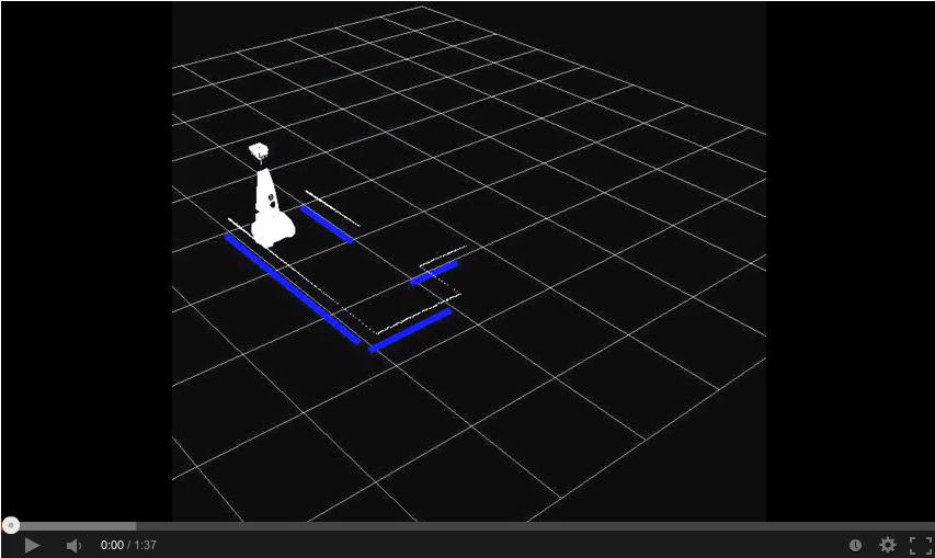
In action
Simulation
Practice
Situation
The situation node is used to detect different types of envriroment.
A few examples are a straight corridor, a side way to the left or a corner at the end of the corridor.
The Situation node first indexes all different types of lines it gets of the line detector.
The first distinction is the direction of a line.
The line can be in the driving direction or perpendicular to the driving direction.
In driving direction
Lines are indexed on base of it's position.
A line at the left side can be behind Pico, line-type L1, next to Pico, line type L2 or in front of Pico, Line type L3.
For lines at the right it's the same except the line types are R1, R2 and R3.
Perpendicular to driving direction
These lines are also indexed on base of it's position.
A line which is only located to the left of Pico is line-type SL, only to the right is of type SR.
If the line crosses the driving direction it is indexed as S0.
The next image makes the location of the different line-types clear.

After the lines are indexed the value of the 3 booleans is decided.
The following flowchart shows how the decisions are made.

After all received lines are categorized a new message is generated for the Localisation node Preferably the lines of type L2 and R2 are broadcast-ed. If these lines are not present, line-types L3 and/or R3 are used.
Deciding the situation according different line-types
When all lines are indexed the upcoming situation needs to be determined.
Localisation
The Localisation node is use to navigate through corridors without touching a wall.
It uses 2 lines as input data which it gets from a message of the Situation node.
The output is a message containing 3 float32 numbers.
The first float32 is the average angle between the driving direction and the 2 lines.
The second float32 is the distance in the Y-direction between the center of Pico and the detected line at the left.
(see picture of used coordinate system above)
The third float32 is the distance in the Y-direction between the center of Pico and the detected line at the right.
Reasoning
The reasoning module is responsible to solve the maze. For this task the module uses the wall follower algorithm also known as the left-hand or right hand-rule. The principle of wall follower algorithm is based on always following the right wall or always following the left wall. This means that the wall is always on your right hand for example (see picture maze). If the maze is not simply connected (i.e. if the start or endpoints are in the center of the structure or the roads cross over and under each other), than this method will not guarantee that the maze can be solved. For our case there is just one input and output on the outside of the maze, and there are also no loops in it. So the wall follower algorithm is in our case very useful.

The reasoning module gets information from the previous module about the next decision point. These decision points, are points where a decision should be made for example at crossroads, T-junctions or at the end of a road. At the decision points, the reasoning module determines the direction in which the robot will drive, by using the wall follower algorithm. For example when module gets information about the next decision point, which is a crossroad, then the reasoning module determines that the robot turn 90 degrees at this point so that the robot following the right wall. There also comes information from the vision module this module, search to arrows on the wall. This arrows refer to the output of the maze and help to solve the maze faster. When there is relevant data from the vision module, this data will overrule the wall follower algorithm.
Motion

The motion node consists of three parts: signal interpolator, motion planner and the drive module. Al this parts determine dependent of the input signals (actual position and target position) the drive speed and rotation speed of the Pico robot.
Signal interpolator
The goal of the signal interpolator is twofold. First, it provides a steady fixed rate of information for the other modules in the local planner. Secondly, it provides relative information between actual data form localization and reasoning. It does so by combining data acquired from the localization and reasoning module with the odometry data from the encoders. Herein the data from localization is presumed to be ideal, meaning the data is always correct. However both types of data are given in different frames.
The localization and reasoning data is provided relative to the corridor section the robot is currently in. Localization gives the distances to both the left and right wall as well as the angle between the corridor and the robot orientation. Reasoning provides the distance to the decision point and the action to be taken there.It can be seen that when localization data is not provided, information is desired about these parameters based on the odometry data.

The odometry data cannot be represented in an external frame by definition. Therefore this data is the relative position of the robot with respect to the start point. This data is calculated by measuring the angle of the wheels over time. Consequently loss of traction is not detectable by this data. However is we presume infinite tractions or limited loss of traction we can use the odometry data to interpolate the localization and reasoning data.
To do so we need to transform the odometry data to the frame of the localization and reasoning data. The transformation has to be reset as the robot rounds a corner because this defines the frame of the localization and reasoning data. The transformation consists of two parts, the translational and the rotational component. The translational component is handled by setting an offset in the odometry data based on the localization data. However this offset alone would result in a flip of the x and y axis because the robot has a different orientation in the odometry frame but the same in the localization frame. To adjust the odometry frame has to be turned to match the difference in corridor orientations. This rotation is done using the first sample of localization data when the turn is complete, using the orientation fault to adjust for any errors made in the turn, thus aligning both frames.

The flow of the module can be described by the following diagram:

Motion planner
The motion planner has two main goals. The first one is to navigate the robot between the walls dependent of the input information from the signal interpolator. The second goal is to navigate the robot in the right direction on the decision points. These decision points, are points where a decision should be made, for example at a crossroad. These decision points, and the decision itself, will be determined by a previous module.
Firstly the navigation to stay between the walls, this navigation provides that the robot stays between the walls and doesn’t hit them. To fulfil this task a simple controller is used, which works on the following principle: When the Pico robot stays in the orange zone it always drives forward. During the ride it is possible that the robot will drive a little skewed, for example by friction on the wheels. In this situation the robot will adjust in the correct direction. When it is not possible to send the robot in the correct direction, the robot will drive into the red zone. In the red zone the robot stops driving straight forward and turn in the correct direction, away from the wall. When the orientation of the robot is correct, the robot will drive straight forward.


Secondly the navigation for the decision points. When the robot is inside the border of the decision point the robot will stop driving (the information about the distance up to the decision point itself comes from the reasoning module). On this moment the navigation to stay between the walls is overruled by the navigation for the decision points. After the robot is stopped the robot will rotate in the correct direction, for example turn -90 degrees. When the rotation is done the navigation to stay between the walls takes over and the robot will drive forward until it is on the next decision point.


Drive module
The drive module is meant to realize the desired velocity vector obtained from the motion planner. In the current configuration the desired velocity vector is directly applied to the low level controllers since these controllers causing maximum acceleration. Test on the actual machine must point out whether or not the loss of traction due to this acceleration causes significant faults in the position.
Software development
Theory
include hough transform here
Usefull links / References
- Information about maze solving: http://en.wikipedia.org/wiki/Maze_solving_algorithm
- Nice java applet about Hough transform http://www.rob.cs.tu-bs.de/content/04-teaching/06-interactive/HNF.html
- OpenCV Hough transform tutorial http://docs.opencv.org/doc/tutorials/imgproc/imgtrans/hough_lines/hough_lines.html