Mobile Robot Control 2023 Wall-E

Group members:

Name	student ID
Lars Blommers	1455893
Joris Bongers	1446193
Erick Hoogstrate	1455176
Noortje Hagelaars	1367846
Merlijn van Duijn	1323385
Sjoerd van der Velden	1375229

Design presentation

The file for the design presentation can be found here:File:Design Presentation Group WallE.pdf

Introduction

For the last several years, restaurants have suffered from a labor shortage. Everywhere around the country restaurants workers are subjected to a heavy workload with no end in sight. In an attempt to resolve this problem, we set out as a group of 6 students to design an algorithm for a robot that can deliver orders to tables. In the span of 10 weeks, we learned all about software design and autonomous robots and immediately put our new knowledge to work in exercises and challenges.

On this wiki page the following aspects of the project are discussed. First, the strategy with regards to the restaurant challenge is discussed. Next, the software architecture and robustness is explained. Finally, the results are evaluated and a conclusion is drawn.

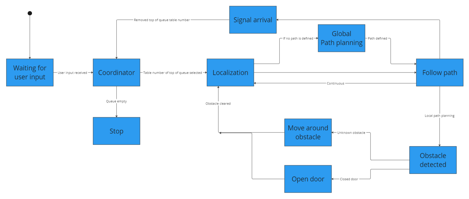
State flow diagram

State flow diagram for restaurant challenge.

The state flow diagram, a type of behavioural diagram, shows the design of the discrete control within the system. They graphically represent finite state machines.

The state flow diagram is a representation of what the blocks in code should do, when a certain input is received or a certain object is detected. The main aspects are worked into this, including the local and global path planning, obstacle avoidance and localization. This gives a rough idea of how the robot should behave.

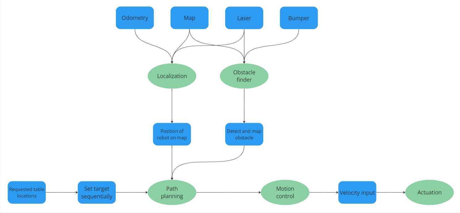
Data flow diagram

Data flow diagram for restaurant challenge.

The data flow diagram shows a structured analysis which gives insights into the origin of the data and interfaces between processes. The diagram consists of data, representing the information, process, which is a functional component with inputs and outputs, and lastly the flow, which specifies an input/output relation between the process and the data.

The data flow diagram uses all data available and the flows point to the appropriate processes in order to execute those parts accordingly with the received data.

Strategy description Restaurant challenge

1.       Initialization:

-       Receive the list of tables to visit in the correct order.

-       Load the provided map of the restaurant.

2.       Localization and Mapping:

-       Use the particle filter as localization algorithm to estimate the robot's position within the restaurant environment.

-       Process the LiDAR data to build and update a map of the environment.

-       Incorporate the static object information into the world model.

3.       Global Path Planning:

-       Use the A* algorithm as the global path planner to generate an initial path from the robot's current position to the first table on the list. The global path consist of waypoints which the robot has to follow

-       Consider the map information, such as walls, doors, and tables, to plan a collision-free path. Doors can be open or closed, the robot should now that where the doors are to avoid local path planning at this location when the door is closed. The robot should make a sound signal to open the door.

4.       Local Path Planning (Open space approach):

-       Continuously check the LiDAR data, for detecting obstacles.

-       If an unknown or unexpected obstacle is detected, switch from global to local path planning for obstacle avoidance.

-       Reassess the obstacle situation continuously and adjust the local path if needed. When using the open space approach the robot will check where the the most room is available and will drive in this direction. When an object suddenly comes too close the robot will totally stop and will wait until the moving obstacle disappears.

-       Reaching a safe region: Switch back to global path planning once the robot reaches a safe distance from the obstacle.

5.     Switching Back to Global Path Planning:

When the decision is made to switch back to global path planning:

-       Pause or slow down the robot's motion temporarily to ensure safety during the planning phase.

-       Replan the global path using the current robot position, updated map information including the obstacle encountered during local path planning.

-       Calculate the new global path as a revised sequence of waypoints to follow.

6.      Table Delivery:

-       Drive the robot to the first table, following the global path.

-       Position the robot near the table. Make sure the robot is facing the table with a suitable range for the order delivery.

-       Use a sound signal to announce the robot's arrival at the table.

-       Wait for a predefined time period to ensure the delivery is complete.

-       Repeat the above steps for each table on the list, following the specified order.

6. Error Handling and Replanning:

-       Errors can occur due to unexpected situations, such as failed table delivery attempts. When this happens, the robot should replan to generate an alternative path or recovery strategy.

-       Replan the global path considering the current robot position, remaining tables, and updated environment information.

Software Architecture Restaurant challenge

Structure of software

In the exercises during the first weeks of the course all seperate elements of the robot control like global and local path planning and localisation were treated. The challenge was then to combine all seperate functions into one executable that can be called with:

./hero_do_your_thing 2 3 4

The folder containing the main executabe file also contains the files from the A*- algorithm (global path planning), the open space approach (local path planning) and the localisation (particle filter). The executable uses multi-threading in order to run the navigation and localisation algorithms in parallel. Two threads are run simultaneously, one calling the function for navigation and one for localisation.

The navigation function first retrieves the table order as arguments and stores it in a table list variable. This table list is then used together with a table nodes list to determine the predefined node in the map that corresponds to the table. The loading of the json file containing the map parameters including the node definitions is hardcoded into the executable. The node list containing nodes that correspond to the tables that have to be visited by the robot is used in a for loop where the A*- algorithm is used to compute a path from the start till end node. For each loop in the for loop the previous end node is taken as the new starting node for the new path. Once the robot had reached the table node it will signal the customer that it has arrived with the io.speak() function. Once the robot notices an obstacle within a set range in its laser data the robot will switch from global path planning (A*- algorithm) to local path planning (Open space approach) and try to dodge the obstacle. After a set time interval the robot will use the node that is closest by to determine a new path using the A*- algorithm.

The localisation function determines the location of the robot on the map using odom data, laser data and information from a png file of the map. The particle filter estimates the current location of the robot and stores this data in a variable. A pointer pointing to the location of this variable is given as an input to the navigation function so the robot can follow the path computed by the A*- algorithm.

Global path planning

- Introduction

Node definition

- Vector map

- Node placement

A*- algorithm

- Algorithm principle/working

- Path following (control)

Local path planning (Obstacle avoidance)

- Introduction

Algorithm selection

- APF vs Open space

Open space approach

- How does function work

Localisation

Localisation is necessary to determine the location of the robot in its environment. Determining the robots location solely on data from the wheel encoders results in a wrong location due to sensor drift and slip from the wheels. Laser data, odometry data from the wheel encoders and information from the map is combined to get a better approximation of the robots current location. Localisation is done by using a particle filter algorithm. The particle filter initialises a set of particles which are possibles poses of the robot on the map. A probability is assigned to each particle after which the weighted average of these particles is taken to determine the most probable pose of the robot. The cloud of particles is constantly propagated through space using the odometry data of the wheel encoders and resampled to get a more accurate approximation.

Particle initialisation

Particle Initialisation

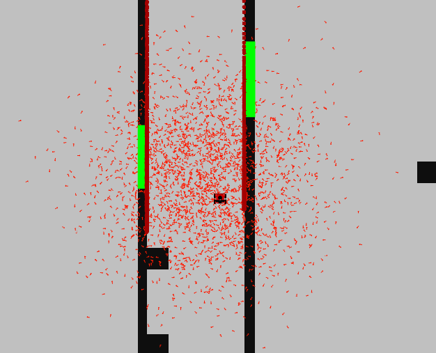
The algorithm starts by initialising the set of particles according to a certain distribution. Each particle in the set represents a hypothesis for the current pose of the robot. The particle cloud can be initiliased either through a uniform or a normal distribution. The particle initialisation through a normal distribution can be seen in the Figure on the right.

Particle propagation

- Propagation on odom data

- Frame transformations

Particle probability

In order to determine the particle that is the best approximation of the robots current pose the algorithm assigns a weight/likelihood to each particle. The largest weight value gets assigned to the particle that has the highest probability of resembling the current pose of the robot. The computation of the weight uses information from the map and the laser data of the robot. For each particle the laser data of the actual robot is compared to the what the laser would have looked like would the robot have the pose of the particle. The theoretical laser data of the particle is computed using a ray casting algorithm for a certain subsample of laser rays (to speed up computational time). The two sets of laser data are compared to eachother and used together with a set of probability density functions to determine the weight of the particle. The probability density functions used are:

1. A Gaussian distribution to account for noise in the laser signal.
2. An exponential distribution to account for an unexpected short reading due to an obstacle being present that is not drawn in the map.
3. A uniform distribution to account for unexpcted long readings due to the laser sensor not retrieving a signal when the laser hits a glass or black object
4. A uniform distribution to account for general random measurements

In this way each laser ray of the particle is assigned a certain probability after which the product of all individual ray probabilites are taken to obtain the weight of the particle.

Resampling

- resampling functions

- Algorithm used and frequency of resampling

Function description

In this paragraph every function is discussed. The input and output data and the way this data is processed are the main aims of this paragraph.

User input

Inputs: User defined sequence of numbers inputted through terminal

Outputs: Array with table numbers in correct order

This is a simple function that requests the sequence of table numbers as a user input. It then converts these numbers into an array where every index of the array is a table number.

Coordinator

Inputs: Array with table numbers, Signal that the robot has arrived at the table

Outputs: Table number, Stop signal

The coordinator keeps track of the table number that the robot has as goal. Once the robot arrives at this table, the coordinator sets the next table in the queue as the new goal. Once all tables have been visited, it stops the robot.

Localization

Inputs: Laser data, odometer data, map data

Outputs: xy position of robot, rotation of robot

This function is the heart of the system. It takes the laser, odometer and map data and combines them to determine the position of the robot with regards to the map. It uses the ParticleFilter as designed in the exercises to achieve this goal.

Global Path planning

Inputs: Node locations, Current position of the robot, Goal table number

Outputs: Sequence of nodes for Path

The global path planning function makes use the A* algorithm as defined in the exercises. It looks at the current position of the robot and calculates a path through predefined nodes. It sends the sequence of nodes that the robot needs to follow to arrive at the goal.

Follow path

Inputs: Location of the robot, Sequence of nodes for Path.

Outputs: control commands for robot

When the sequence of nodes is defined, this function makes sure the robot moves from node to node until it reaches its goal. It uses either the open spaces or artificial vector field approach for this.

Obstacle detected

Inputs: laser data

Outputs: control commands for robot

When an object is in the path of the robot, it needs to be avoided. This function will take care of that. It overrules the path following function.

Signal arrival

Inputs: location of the robot, location of the table

Outputs: Sound message, signal to coordinator to set next table as goal.

This function looks if the robot has arrived at the table by calculation the distance between the robot and the table. Once this value is under a certain threshold, a sound message is sent to the robot and the coordinator is informed that the robot has reached the table.

Task description

Task decriptions

Name	Tasks week 8	Tasks week 9	Tasks week 10
Lars Blommers	1. Localisation (particle filter)	1. Main file state flow	1. Combine different elements in main file 2. Combine A* with localisation
Joris Bongers	1. Navigation (combining global and local navigation)	1. Update wiki with interface, coordinator information	1. Combine different elements in main file 2. Combine A* with localisation
Erick Hoogstrate	1. Localisation (particle filter)	1. Finish up localisation (particle filter)	1. Combine A* with localisation
Noortje Hagelaars	1. Adjust state and data diagram after feedback from tutors 2. Navigation (A* algorithm)	1. Robot implementation of A*	1. Create vector map of final challenge, node placement for A*
Merlijn van Duijn	1. Navigation (A* algorithm)	1. Robot implementation of A*	-
Sjoerd van der Velden	1. Adjust state and data diagram after feedback from tutors 2. Navigation (combining global and local navigation)	1. Update wiki with interface, coordinator information 2. Assist with robot testing A*	1. Combine A* with local navigation