Mobile Robot Control 2023 The Iron Giant
Group members:
| Name | student ID |
|---|---|
| Tobias Berg | 1607359 |
| Guido Wolfs | 1439537 |
| Tim de Keijzer | 1422987 |
| Marijn van Noije | 1436546 |
| Tim van Meijel | 1415352 |
| Xander de Rijk | 1364618 |
| Stern Eichperger | 1281232 |
Midterm presentation
The midterm presentation of The Iron Giant: File:Midterm-presentation-The-Iron-Giant.pdf
The feedback and questions received regarding the midterm presentation of The Iron Giant are as follows:
Feedback point 1:
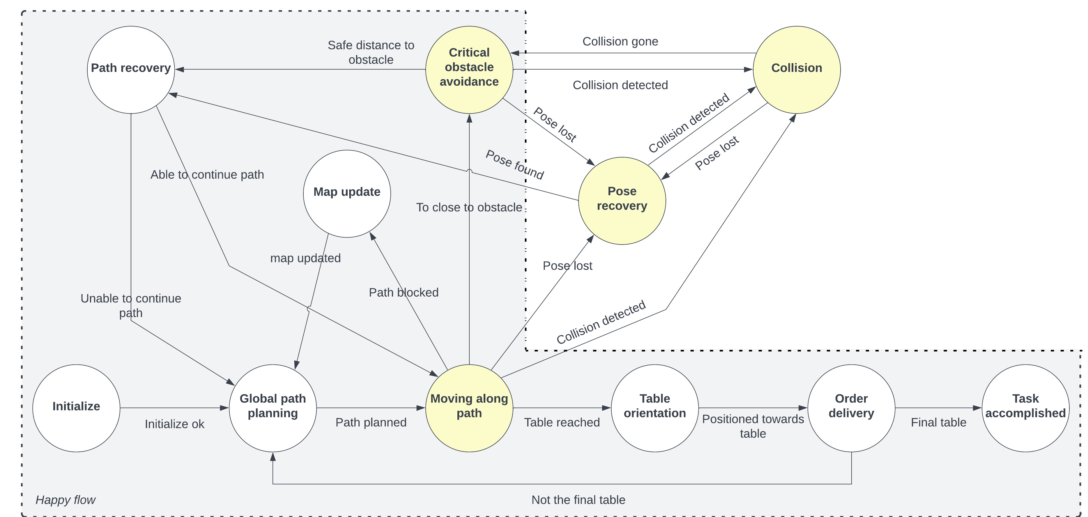
- The current state diagram does not include a recovery state to resolve a deadlock situation. If a passage suddenly becomes blocked and remains blocked, the robot could potentially end up in a deadlock. This could occur, for example, if a person obstructs a pathway between obstacles and does not move away.
Solution: To address this issue, an additional recovery loop should be added for handling suddenly blocked pathways. In this loop, the obstructing obstacle is added to the map, and a alternative new path is calculated using the A* algorithm.
Question 1:
- How does the robot transition into the pose recovery state? What parameter or condition is used?
Solution/answer: A condition based on the standard deviation of the particle spread should be implemented. If the deviation is too large, indicating a significant spread of particles and therefore an uncertain estimation, the robot has lost knowledge of its position in the world and needs to recover it.
Question 2:
- Why was the "happy flow" defined in this manner? Won't the robot always encounter disturbances and dynamic objects that cause it to loop through parts of both the happy and unhappy flows? In such cases, the loop may not necessarily be considered an unhappy flow.
Solution/answer: It is true that the definition of the happy flow was somewhat rigid. It is true that certain segments of the "unhappy flow" may occur within the expected states the robot will loop trough during the challenge. This does not pose a problem and does not represent an unhappy flow.
We updated the state diagram according to the feedback and questions as shown in Figure 1.
Final Challenge
Introduction
In this project, the goal is to successfully drive the Hero robot to a table in a restaurant, using a predefined map, with unknown static and dynamic obstacles. To apply the developed code to the Hero robot, the C++ programming language is used. The goal is to enable the Hero robot to navigate and locate itself within the environment. Localization and navigation are two aspects of autonomous robots that will be focussed on.
For a robot to drive autonomously, it is important the robot knows its current location and orientation. This requires localization of the robot. This localization method must be based on a predefined map, but should also compensate for partial imperfect situations (living in the real world). The key idea of localization is to have a map of the environment and sensor measurements, which is used in a so-called particle filter to get a better localization of the robot pose. This particle filtering method uses a probabilistic approximation of particles, each representing a possible hypothesis for the robot position.
Next, the robot must be able to navigate itself to the desired position by following a certain path. To plan the path of the Hero robot, the A* path planning algorithm is used to calculate the most optimal path for the robot to effectively reach its destination. This is the so-called global navigation the robot uses. In addition, the local navigation allows the robot to effectively navigate through the map and avoid obstacles in real time. To account for the objects in the final challenge, the so-called artificial potential field method is used.
To complete the final challenge, localization and navigation techniques must be combined. By developing the software for the final challenge, the robot will identify its location on the map, plan an optimal path and complete the task by moving precisely to the designated table. This wiki page thoroughly describes these algorithms and explains how they are implemented. In addition, it discusses how these algorithms interact and their performance and robustness is determined. An evaluation is given at the end, with a conclusion, discussion and future steps.
Strategy description
Hoe willen we het gaan bereiken Beschrijven dat we deuren willen toepassen, en in het hoofdstuk robustness omschrijven welke moeilijkheden we zijn tegenkomen
Algorithms used
A star
For the global path planner we use the A* algorithm with some adjustments. Initially, the particle filter determines the input in map frame in meters. This is converted to pixels for the input of the global planner. Goals are predefined in pixel positions and are also given as input for the planner. For robustness first the node list is calculated after which the closest node for those pairs of pixels is used as entrance and final node.
For calculating the node list, we read the image of the map with gray scaling. Since pixels can be either black (0), gray (128) and white (255), these values serve as threshold for squeezing values to binary values. Another input of the global planner is a list of which doors we want to use. Each door has a cluster of nodes, which are then used for updating the map after thresholding depending if they serve as wall or not. Similarly, with use of the particle filter and the laser data, the objects are converted from meters to pixels. A min and max function is applied to ensure all laser point locations are within the map and are then added to the obstacle map, separate from the map with walls and “closed” doors. For added robustness a margin of a 15 pixels is applied for which an open node needs to be away from walls and obstacles. Each node is defined on a grid from the map with a defined step size of pixels, in this case 10 pixels per step size.
With the remaining node list, a list of connections for each node is made in the directions, up, down, left, right and diagonal.
Before running A* the position and distances from the goal are computed in map frame. An additional cost function is defined for every pixel near a wall or obstacle. If it is within a range of 20 the node has a high cost of 100, whereas within 30 in has a low cost of 2.
For A* we take with every step the node with the lowest cost-to-come. For this node, it will add all connected nodes and applies the lowest cost-to-go. The cost-to-go is determined by the step size from one node to the next (meaning going to a diagonal node has a higher cost) with addition of the added cost of being near a wall or obstacle for the node-to-go. After A* has reached the final node, it will create a path in map frame in meters. Since the distance between nodes is small, the new path is every third step of the full path. This is then send to the local path planner.
For visualization after each time it has found a path towards a goal it will make an image plotting both the walls, doors, path and obstacles in respective colors black, gray, red and blue. Each time the global path planner is run a new image is made, not overwriting the previous one.
Similar to the A* algorithm, the Dijkstra algorithm is used to determine which nodes are a door. By putting the algorithm in a for loop of the nodes that are a door, it is possible to cluster all node positions per existing door. The reason for doing this is because it makes it robust if we want to make a path through one door but not the other. The node list is determined similarly as previous by applying a threshold on the image and finding the nodes of the door. It is sufficient to only look in the directions up down, left and right for the node connections. This information is also used as input for the global path planner.
Particle filter
A particle filter is a commonly used probabilistic filtering technique in robotics that estimates a robot’s pose based on sensor measurements while navigating in an environment. The presence of wheel slip and noisy data causes imperfections in the odometry data, therefore it is not possible to fully rely on the odometry data to get an accurate enough estimation of the robot’s pose. In order to get a better estimation of the pose of the robot while it is going to the tables in the restaurant, it is important to implement a localizing algorithm that estimates the pose of the robot on the map. Therefore, a particle filter algorithm is used in the final challenge.
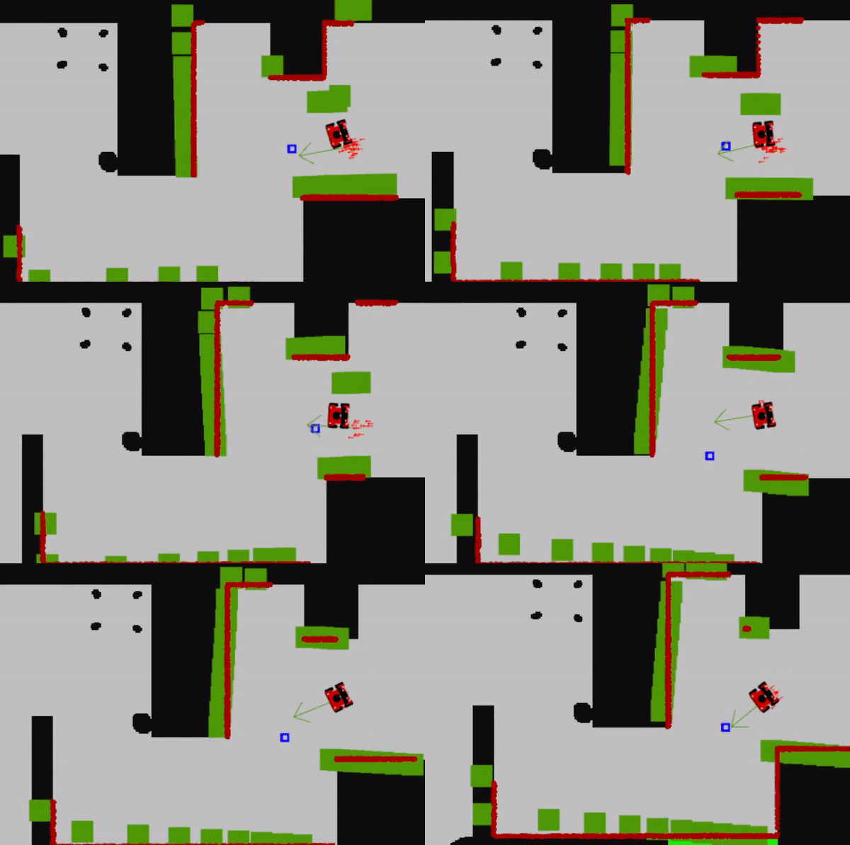
The particle filter made in the previous assessments forms the bases of the algorithm that was eventually implemented. In this algorithm, each particle describes a hypothesis of the current pose of the robot. At first, the particles are distributed with a Gaussian distribution around the robot, resulting in a broad range of the potential pose of the robot, see Figure 4. Based on the lidar and odometry data of the robot, the particles are resampled with weights based on the likelihood of their pose. This is done by a filter that approximates the probability distribution of the robot’s pose. A “Recursive State Estimation Beam-based model” is implemented that computes the likelihood of each measurement given a prediction. This model accounts for measurement errors including, measurement noise, unexpected objects, errors due to failures to detect objects and random unrecognized noise. Finally, the particles will be resampled so that high likelihoods are represented heavily in the new particle set. A multinomial resampling method is used. This method selects particles based on their weights, emphasizing particles with a higher likelihood of representing the true pose. This results in a final estimation of the robot’s pose.
For the restaurant challenge, the particle filter is updated during each iteration in the main “while loop”. Updating the filter during each cycle ensures smaller differences in robot poses, making it easier for the particle filter to update and predict a more accurate pose when the robot moves. To increase the computation speed, the number of particles was slightly reduced together with a higher subsample value of the laser data.
Artificial potential field algorithm
Local navigation utilizes an artificial potential field algorithm which was used before during the preliminary assignments. The artificial potential field algorithm is based on the principle of artificial repulsion from obstacles and artificial attraction towards a goal. These repulsions and attractions are then combined to generate an artificial resulting force which indicates the motion direction of the robot. This method aims to draw the robot towards a certain goal while avoiding obstacles on its path towards that goal.
For the implementation of the artificial goals, the path goals calculated by the A-star algorithm are utilized to set the direction of the artificial attraction force. The magnitude of the force is kept constant over the range towards the goal. As the robot progresses, it visits each path goal one after another, updating the artificial attractive force to the next goal upon reaching its local path goal. The artificial repulsive forces of the obstacles are based on the detection of these obstacles by the laser sensor. Laser beams detected within a certain boundary are converted to artificial force vectors pointing towards the robot resulting in repulsive forces. The magnitude of the forces is based on the detected length of the laser beams. The forces are scaled by the distance of the detected obstacle to the robot with an increasing force for a decreasing distance. Additionally, the repulsive forces are split up into two laser beam angle ranges, a range representing the front part of the robot and a range representing the sides of the robot. The repulsive force vectors in front of the robot are assigned a lower weight compared to those on the sides.
This implementation of the artificial potential field algorithm has several advantages. First of all, the laser beam detection allows for the navigation around dynamic objects and in dynamic environments where obstacles may move or appear unexpected. Furthermore, the algorithm is relatively computational efficient allowing real-time navigation. Splitting up the repulsive forces in a front and side region allows the robot to navigate around corners and obstacles with a larger margin. A drawback of this method is the swaying of the robot when it is trying to move through small corridors or between objects which create a small passage. Another drawback of the artificial potential field algorithm is the problem of getting stuck in local minima like corners. This resulted in the need of additional methods to navigate out of these local minima and get back to a viable path.
Software Architecture
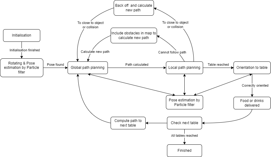
First, individual components were designed for the final challenge. However, it is important to combine them in a structured way. It was decided to create one main file in which all the individual components are implemented. The different components are called by using functions. This way, the main file remains clean. In the main file, a while loop is used to repeatedly run the desired functions. To determine which parts of the code have to be run, a ‘switch’ is implemented, using ‘cases’ for different states of the robot. By using booleans and ‘if’-statements, the next state can be chosen. In this way, a state machine is created. Obviously, the states involve a lot of safety-related conditions. Firstly, the initialisation starts by running the particle filter (case A) while the robot turns left and right. By doing this, the environment around the robot can be better perceived and the particle filter gives a better approximation of the initial pose.
Secondly, when initialization is complete, the code proceeds to case B. In case B, the code calls the A* algorithm to calculate the optimal path. When case B is reached after case A, the A* algorithm will determine the optimal path starting from the robot's initial position determined by the particle filter. Case B can also be reached from other cases, this means, for example, that the robot has detected an object and cannot continue its path through its previously defined path. In that case, the A* algorithm is recalculated from its current position, taking into account the object it has detected via laser data. If the robot needs to reach several tables in succession, it first calculates the optimal path to the first table. Once the robot has reached that table, it will return to case B and run the A* algorithm to the next table.
Next, when the global path has been determined in case B, the local path planner will take over to reach the desired table in case C. The local path planner makes use of the intermediate steps which have been determined by the A* algorithm while taking into account objects. These objects have a repulsive force on the robot which reduces the chance of collision. The intermediate goals have an attractive force on the robot. This means the robot has a preferred direction it wants to drive in, which will lead to the final goal which is the table.
During this state, the particle filter is run iteratively with the local planner. This means the pose of the robot remains accurate.
When an object comes too close to the robot, it will trigger a safety mechanism which will make sure the robot does not collide. The robot will then go back to state B and plan a path around the object by taking into account the found objects in the laser data, as mentioned before.
When the robot is close to its final goal, thus close to the table, the speed of the robot will reduce. This makes sure the approach to the table is smooth and safe. The script then switches to case E, which ensures that the robot orientates itself to the direction of the table. The food and drinks can now be picked up from the robot.
When all tables are reached, the main code switches to case D. In this case, the while loop breaks and the code stops running.
Performance
Robustness
Conclusion
Wat hebben we bereikt
Discussion
Discusseer wat verbeterd kan worden
Future steps
Future steps will describe some follow-up steps if one wants to continue with the current code.
As described earlier, one of the first obvious future steps would be to implement the option to pass through a door. Right now, this still has some implications, especially with the particle filter. The problem right now is that the map is not updating correctly. When you go through the door, there are no walls, while the particle filter still thinks there is a wall, because of the predefined map. Therefore, the particle filter no longer indicates the correct robot position when the robot passes through the doorway. The first future step will be to fix this bug and ensure that the particle filter can handle opening the door, for example, by updating the map that the particle filter uses.
Another future step could be to make the robot move more smoothly. The robot sometimes moves a bit restlessly.


