Mobile Robot Control 2023 Group 4

Group members:

Group 04

Name	student ID
Lowe Blom	1266020
Rainier Heijne	1227575
Tom Minten	1372300

Exercise 1: Don't crash (video link):

https://drive.google.com/file/d/1zgMMQwU3ZrADZJuFCLglQiefVecF3_95/view?usp=sharing

Exercise 2: A* algorithm

• The code can be found on our gitlab page
• The middle nodes in a straight line without more than two neighbors can be removed. Since the speed of the algorithm is O(n) with n the size of the grid, removing cells from the grid will improve the performance of the algorithm.

Exercise 3: Navigation through a corridor

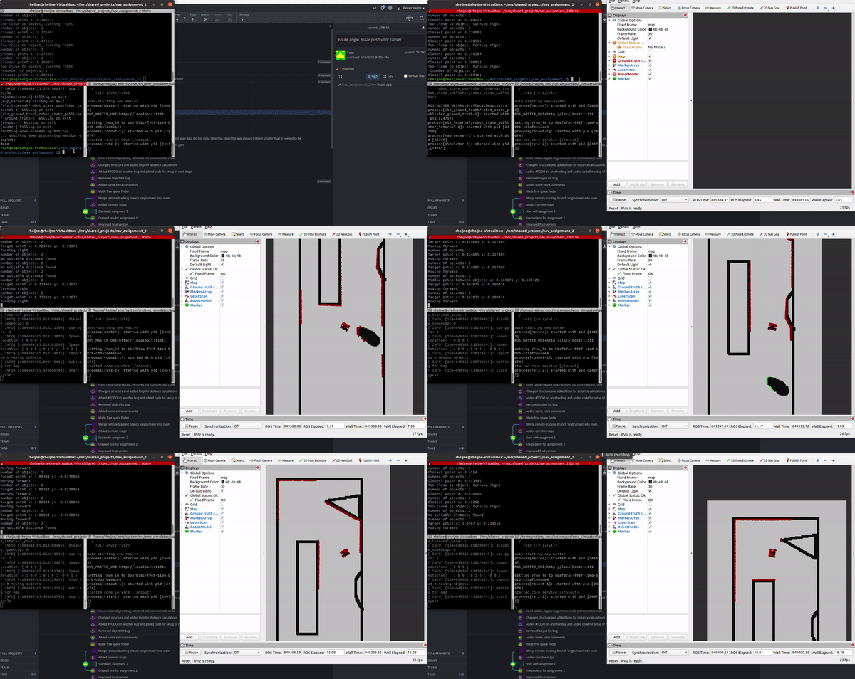
The robot has to drive 5 meters through a corridor with a width of 1 to 2 meters, without a collision with present obstacles. Our solution is based on looking for free space around and between objects. The following steps are taken for each laser data set:

Simulation of the robot driving through a corridor with obstacles

1. Laser sensor data is read to detect obstacles.

2. Detected obstacles are stored in a list of objects with all the relative positions of the scan points of each object.

3. The code identifies the boundaries of the each detected object.

4. If there are at least two detected objects, the code finds the shortest distance with a minimum width between neighboring obstacles.

5. The target point is set as the middle point of the largest gap between all objects

6. Based on the target point's position, the robot's linear and angular velocities are set

7. If no suitable distance is found or only one object is detected, the robot  drives straight and turns away if an obstacle gets too close to avoid collisions.

Exercise 4: Localization assignment 1

Assignment 1: Keep track of the location

The code for assignment 1 can be found on gitlab. This code prints the odometry data and the difference between the previous and the current odometry data.

Assignment 2: Observe the behaviour in simulation

By driving in a straight line forwards in simulation with the command: io.sendBaseReference(1, 0, 0); without uncertainty in the odometry sensor will result in a predictable increase in x position of the robot and no change in angle or y value of the odometry data. However in real life the data from a sensor always has a certain measurement uncertainty and the wheels can slip, leading to a different coordinate estimation based on the odometry compared to the actual position of the robot. In simulation the distance driven that is estimated by the odometry object. However, the laser scan data can also be used to estimate the distance that is driven. A block is placed in front of the robot and the difference in scan data between the previous and the current time step is added to a memory variable that stores the distance driven. This value can be compared to the one stored in the odometry object.

By driving straight forward without uncertainty in odometry data the following is observed in simulation:

- The angle and y-value in the odometry data is not changing and remains 0.

- The difference between the driven distance calculated with the scan data and that of the odometry data is quite accurately matching.

By driving straight forward with uncertainty in odometry data the following is observed in simulation:

- The angle and y-value in the odometry data is changing with small increments and thus does not remain constant.

- The difference between the driven distance calculated with the scan data and that of the odometry data is now bigger.

This proves that only relying on the odometry data for position can lead to uncertainty and errors in pose estimation. So it is recommended to use multiple sensors in the final challenge to make multiple estimations. By combining these estimations the uncertainty and error can be greatly reduced.

Exercise 5: Localization assignment 2

Assignment 0: Explore the code base

- Difference ParticleFilter and ParticleFilterBase and relation

- Relation ParticleFilter and Particle classes

- Difference between propagation method of ParticleFilter en Particle

Assignment 1: Initialize the Particle Filter

- Difference between constructors

The first constructor passes the world, weight and a generator pointer to the particle class, which then estimates a pose based on a uniform distribution, whereas the second constructor passes the world, mean, sigma, weight and a generator pointer to the particle class, which then estimates a pose based on a gaussian distribution using the mean and standard deviation.

- Completion of constructors

In ParticleFilterBase a for loop is used to call the particle constructor and place the particle and its location in a vector called _particles for both constructors.

The particle constructor is finished by calling get_noise_sample_uniform() and get_noise_sample_gaussian() for x, y and theta and then using these estimated values to generate an estimated pose which is then initialised.

- Validations

- Advantages/disadvantages of first constructor + second construcor

- When to use both?