Mobile Robot Control 2023 Group 16
Group members:
| Name | student ID |
|---|---|
| Marijn van Noije | 1436546 |
| Tim van Meijel | 1415352 |
Practical exercise week 1
1. On the robot-laptop open rviz. Observe the laser data. How much noise is there on the laser? What objects can be seen by the laser? Which objects cannot? How do your own legs look like to the robot.
When opening rviz, noise is present on the laser. The noise is evidenced by small fluctuations in the position of the laser points. Objects located at laser height are visible. For example, when there is a small cube in front of the robot that is below the laser height, it is not observed. When we walk in front of the laser, our own legs look like two lines formed by laser points.
2. Go to your folder on the robot and pull your software.
Executed during practical session.
3. Take your example of dont crash and test it on the robot. Does it work like in simulation?
Executed during practical session. The code of dont crash worked immediately on the real robot.
4. Take a video of the working robot and post it on your wiki.
Link to video: https://youtu.be/4mXdJyXXidE
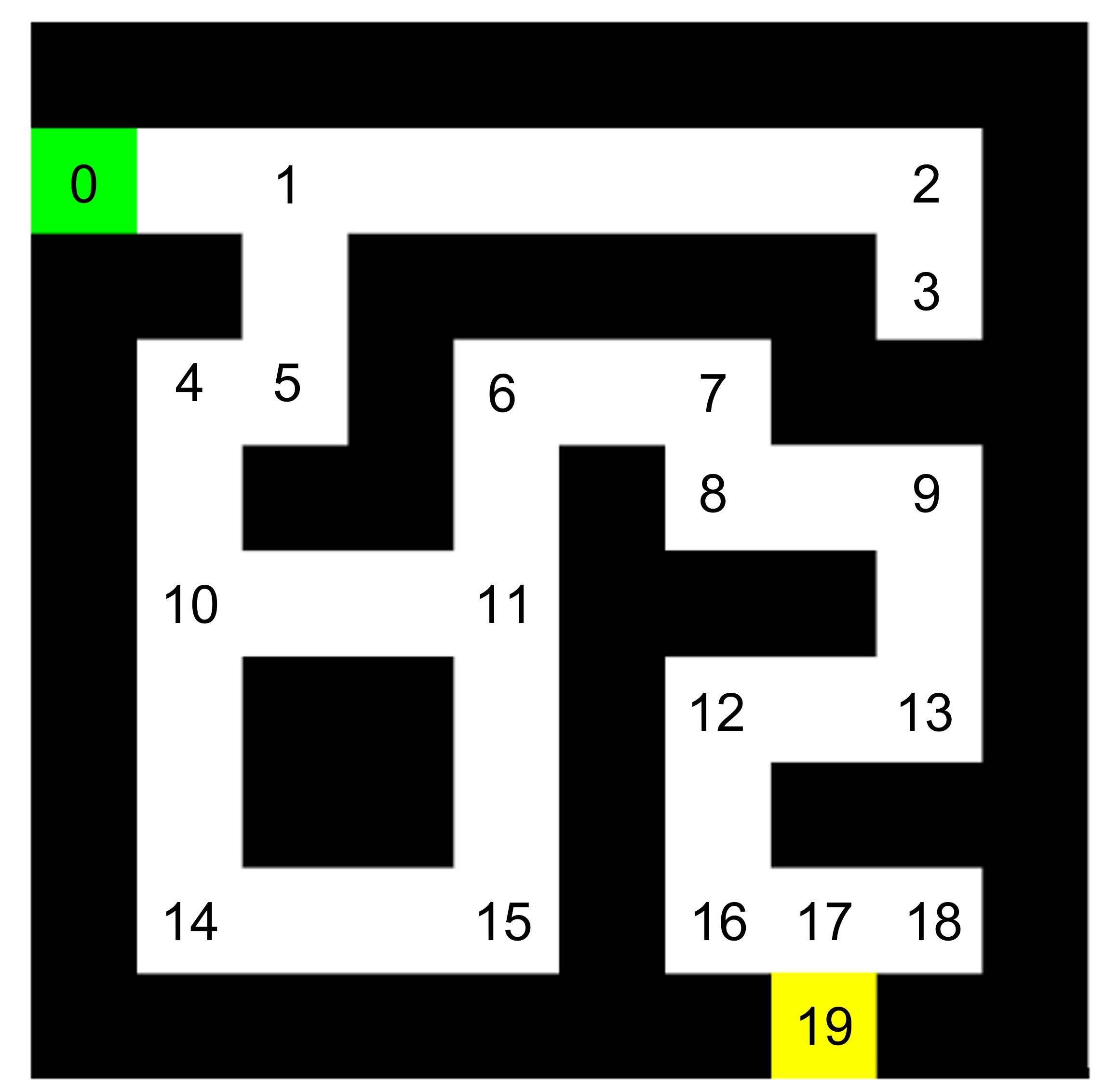
To make the A* algorithm more efficient, the amount of nodes should be reduced. This means that only nodes where the route change direction or where a path ends are considered. This is on the corners, T-junction and cross roads.
This would be more efficient, since the nodes in-between do not have to be considered by the A* algorithm. This increases computation speed.
To move the robot through the corridor, the Artifical Potential Field algorithm is used. There are two types of forces in this algorithm: the attractive force and the repulsive force. The attracting force calculated based on the position of the goal in comparison to the position of the robot. The repulsing forces are calculated by laserdata from walls and obstacles. When the robot moves forward in the corridor, it uses the laser to scan where the objects are positioned. Objects within a range of 1.5 meter are used in our approach. The repulsive forces result in a direction vector in which the robot wants to move. This direction is added up to the direction vector of the goal. Combined, these vectors result in a final direction vector in which the robot wants to move. The angular speed is then set to reach the desired direction.
Link to video of the simulation results: https://youtu.be/TG1GS70-G0A
Link to video of the real life experiment: https://youtu.be/_o3tM3mlx3E
Localisation assignment 1
Assignment 1: Keep Track of our location
Assignment 2: Observe the Behavior in Simulation 1) The accuracy of the odometry data will be evaluated by running a simulation where the robot should follow a square path. The robot will start in the zero position. By following a square it means that when the robot completed the path it should return in its original position. By following the squared path it we can check the odometry data whether this is indeed equal to the zero position or whether the robot knows where he is at that moment. Due to some delays in the odometry data it will probably never return exactly to its zero position, but when the odometry data returns values that are indeed not the zero position, but the position where he really is at that moment, it can be concluded that the accuracy is good. When the odometry data returns diffent values than the position where the robot actually is, the accuracy is perfect anymore.
2) When using the regular odometry data, the path followed will be exact and after completing the path the odometry data returns the exact position of the robot. When using the uncertain_odom it will result in a different position of the robot after completing the path. This is caused due to some slip and disturbances. When for example the first corner is not exactly correct, its next corner will have the error of the first corner plus its own error. This means that by trying to follow the path using odometry data, there are some accuracy issues. So, it is hard to rely on the odometry data.
3) No, we will not use this approach in the final challenge, because in reality the same thing happens when using the uncertain_odom. The accuracy will become more worse over time, so for the final challenge this in not wanted.
Assignment 2: Observe the Behavior in Simulation
