Mobile Robot Control 2020 Group 10

Team members:

Arend-Jan van Noorden (1378147)

Sjors Boutkan (0938234)

Jeroen van Meurs (0946114)

Koen van Gorkom (0954964)

Friso Buurman (0906665)

Escape Room

Design Document

The design document of group 10 can be found here.

Strategy

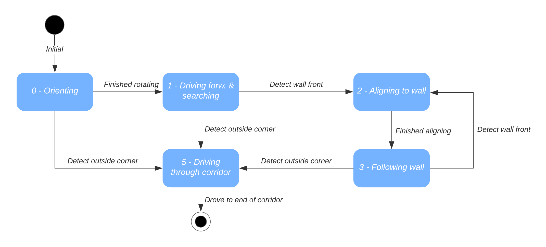
Solving the escape room is quite simple: find the corridor and drive through it. This document givesan overview of the system being build to solve this task.Finding the corridor is done by detecting the two outside corners marking the start of the corridor.Since the room is square, no other outside corners will be present in the environment. If these cornerscan’t be found from PICO’s initial location, it’ll follow the walls of the rooms clockwise, until thecorridor (outside corners) are encountered. The corresponding state diagram is shown in Figure1.1. The movement and navigation will be done using set-points and a potential-field algorithmpreventing PICO from hitting any obstacles or walls.

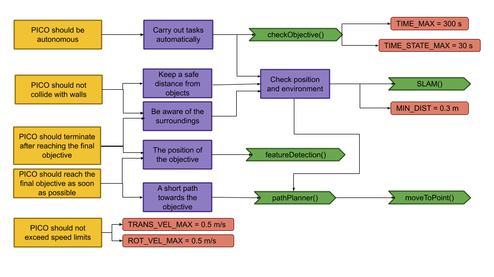
Requirements and Specifications

Links between requirements, functions and specifications.

Requirements	Specifications
PICO should not bump into walls	PICO's measurements are 0.41 m in width by 0.35 m in length
	The free radius around PICO should be at least 0.21 m
PICO cannot exceed speed limits	Maximum translational velocity is 0.5 m/s
	Maximum rotational velocity is 1.2 rad/s
Since PICO will be autonomous, it should be aware of its surroundings.	PICO should have an accurate map of its surroundings.
	LRF range is between 0.01 m and 10 m.
	LRF FOV is from -2 to 2 rad, measured over 1000 points of equal increments.
PICO should terminate when the final objective is reached.	PICO should come to a stop after it has crossed the finish line.
PICO should reach the final objective as soon as possible.	PICO should cross the finish line within 5 minutes.
PICO should not end up in a live lock state.	PICO should not keep repeating one action for over 30 seconds.
PICO should not end up in a dead lock state.	Careful coding has to be done to have no dead lock states.

Components and Functions

Basic architecture of robot code:

State machine of the control strategy for the maze challenge.

All functions need to be run based on a Finite State Machine. As with sensors, all data has noise so these data streams need to be filtered.

The tasks of each component can be divided in several functions each with a specific subroutine.

World model

The world model stores the information gathered by the components and distributes this information to the other components. The information consists of:

• A map of the surrounding area.
• A list of found features.
• The current and previous state.
• The next position to travel to.

The world model contains no functions because the world model is only used to store the world data, so there are no active subroutines present.

Plan

The plan component uses data from the world model to determine the next position PICO needs to go to. It thereby also check if the objective is met.

• checkObjective()
  The checkObjective function is the supervisor of the complete system. It controls/executes the states as defined in figure \ref{fig:state-machine} and executes the strategy as described in \ref{sec:strategy}. It will also check for failure of the system by identifying incorrect states, e.g. not moving for a set amount of time, following a wall for too long or having made a complete loop of the room without finding the corridor.

• pathPlanner()
  The plan component contains the path-planner function, this functions is responsible to define the setpoints for PICO. These setpoints will be determined based on the state machine and the world model.

Control

The control component makes sure PICO moves along the planned path.

• moveToPoint()
  The move to point function will be used to move PICO to the set point generated by the path planner. To prevent that PICO will hit the wall, the world model will be used to determine the trajectory from the current position of PICO to the set point.

Monitoring

The monitor component will try to identify features from the world model data.

• featureDetection()
  To determine the corners and walls of the maze the feature detection function will be used based on the world model data.

Perception

The perception component will gather the sensor data, clean it and update the world model with it.

• getLaserData()
  To acquire the data points of the laser sensor, the get laser data function will be used. The gathered data will be preprocessed to filter out the disturbances. The processed data will be written to the world model.

• getOdomData()
  The odometry date will be read out with the getOdomData function. This date will be written to the world model.

• SLAM()
  The gathered data from the laser and odometry sensors will be used to generate a map of the environment using Simultaneous Localization and Mapping (SLAM)

• UpdateVisuals()
  A window will be opened that shows all the detected features and the path that PICO is going. This function will update that window

Interfaces

All components interface with the world model, getting data required for their functions and setting data created to be used by other components. The world mode is the central data store. This can also be seen in figure Figure Boven. Differences between the the proposed system and the system originally shown in , is that there are no interfaces between the 'resources' and 'capabilities' and the world model. The world model will not be able to get it's own data or control the motors of the system. The interface to the sensors will be through the perception component and the controlling of capabilities will be done by the control component.

Challenge result

Sadly we did not manage to get out of the escape room, below we will discuss why and how we solved it.

Main

After the Maze challenge we analyzed which part of the main program caused the failure which lead to the the wall collision. The problem occurred in the corner detection function, which resulted in the interpretation of a inside corner as an outside corner. The planning algorithm used this corner as target position to search a second outside corner, and let the robot drive to this corner. With the absence of a potential field algorithm, the robot was able to drive through the wall.

The main program for the maze challenge is using the state machine as shown in the Components and functions paragraph, in the following paragraphs is the robot behavior at each state described.

• ORIENTING

In the first state the robot will turn to check if it can see a door or a outside corner. A door is defined if there are two outside corners within 0,5 m and 1,5 m from each other, or a outside corner and a wall within the same range as with the outside corners. If the robot is not able to find a door from its initial position, then there will be searched for a single outside corner. When there is no door or outside corner found then the robot will search for the closest wall to follow.

• SEARCH_FORWARD

If the robot cannot detect any features in the orienting state, then the robot will drive straight forward in the same direction as the initial orientation.

• ALIGN_TO_WALL

When multiple walls are detected the closest wall is determined, the angle between the wall and the robot will be computed to determine the rotation direction. When the robot is aligned within +/- 3 degrees the state will be set to FOLLOW_WALL.

• FOLLOW_WALL

The robot will follow the wall at 20 cm distance till a door or outside corner is found, if this is the case the state will be set to GOTO_DOOR or SEARCH_DOOR. Otherwise the robot will follow the wall if a second wall in front of the is found, when this second wall is closer by then the first wall the ALIGN_TO_WALL state will be called again.

• SEARCH_DOOR

If one outside corner is found a way point will be set 25 cm from the x and y direction with respect of the corner, with this way point there can be guaranteed that the robot will not collide with the wall. When the robot is at this position and the second outside is still not found it will to ORIENTING again, otherwise the robot will be set GOTO_DOOR.

• GOTO_DOOR

When the door is found the planning script will place a way point 25 cm in front of the midpoint of the door, if the robot is at this location the robot will be set to the DRIVE_THROUGH_DOOR state.

• DRIVE_THROUGH_DOOR

In this state the robot will drive to the way point 25 cm in the middle the door, when the robot loses the door the DRIVE_THROUGH_CORRIDOR state is set.

• DRIVE_THROUGH_CORRIDOR

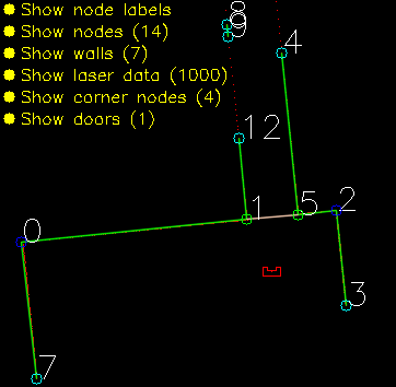
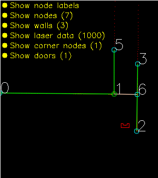
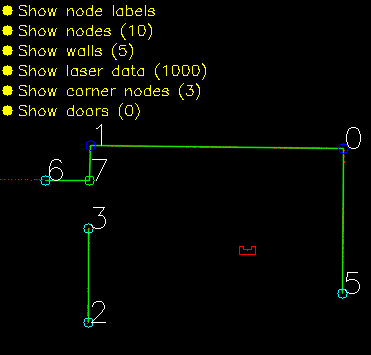
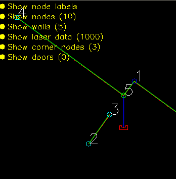
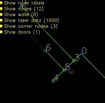
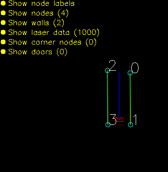
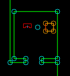
To complete the maze a way point is set in the middle of the furthest corridor walls nodes. To determine the corridor walls there is checked if the walls are parallel to each other, if the perpendicular distance is between the 0,5 m and 1,5 m and if at least two wall nodes can be projected on the other wall to check if the walls are not after each other. When the robot is at this way point the robot has exited the maze and the state will be set to COMPLETED. Below there is shown that the robot is executing SEARCH_DOOR, GOTO_DOOR and DRIVE_THROUGH_CORRIDOR.

Backup

The maze challenge backup attempt. The current state of the state machine is visible in the picture.

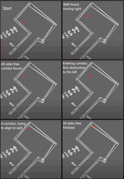
The backup was a simple wall following algorithm. Initially, Pico will drive forwards until it encounters an object in front. Next, Pico will turn 90 degrees to the right. Then, as long as Pico's left side is obstructed, the wall will be followed while making adjustments to align with the wall and not strafe too close to the wall or too far away from the wall. Again, when the front is obstructed as well, Pico will turn 90 degrees to the right and the next wall will be followed. When a gap at the left side is detected, Pico will move forward a little bit, turn left and drive forward into the corridor. If the senses a object in front, Pico will know the opening was only a small gap and not the corridor, in this case Pico will rotate right and continue following the wall.

Unfortunately, the backup attempt failed as well. The problem Pico encountered during the challenge was an edge case which unfortunately did not result in a correct execution of the algorithm. After finding a wall at the front, Pico turned 90 degrees to the right. After the turn all sides were 'free', meaning that Pico thought he was next to a corridor. After turning left it noticed that its front was free and its left side was not. This triggered the state machine to believe it was in the corridor. When the state machine enters this state, the only possible state is the finished state. So after driving through the wall, all sides of Pico were 'free' again thus entering the finished state. Pico drove through the when it thought it was in the corridor. This is because of the specific laser beams that Pico uses for the collision detection. Pico checks three sides, using ten laser beams per side. The front side is the actual front of Pico. The right and left side however, are about 45 degrees from the front instead of 90. Since the actual side of Pico was not monitored, Pico thought he was still some distance away from the wall.

After the challenge a little time was spend to improve the behavior of the wall following algorithm. To this end, the hard 90 degree turns have been replaced by an alignment check and the collision detection was changed that the actual right and left side of Pico are measured. When an obstructing in front is detected, Pico rotates until the obstruction is not visible anymore and the left side is aligned to a wall. This is checked by comparing the ranges of a subset of the of the LRF to the left of Pico. When the ranges are about equal, Pico is aligned. With this improvement, Pico was able to reach the actual finish of the Maze Challenge.

Hospital challenge

Components [Friso]

World model [Koen]

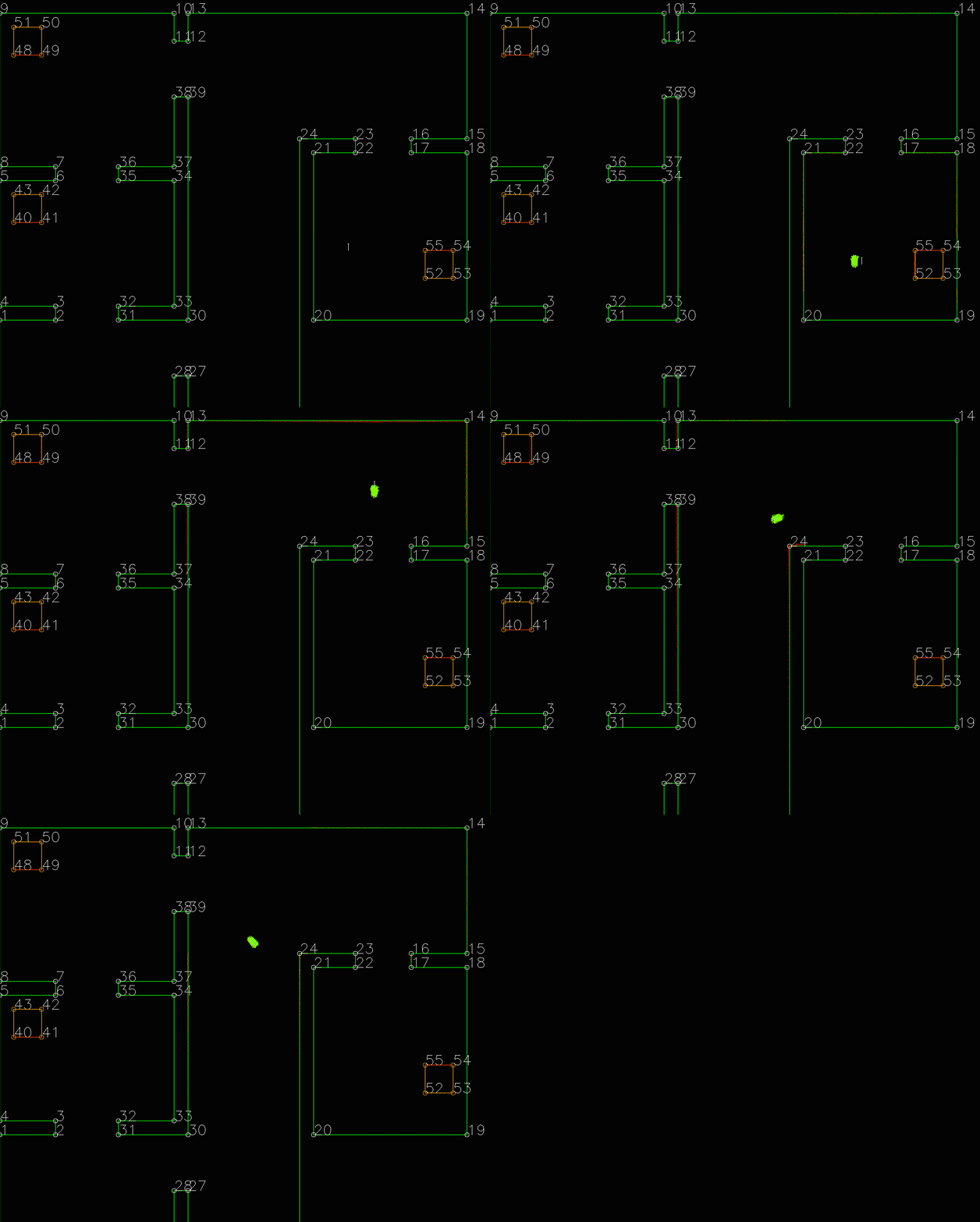
The world model is used as a database. This database is separated into two maps: A global map and a grid map. All gathered data is stored in the world model and then can be used by other processes. Besides the data structure the world model also has a couple of functions to update the model and extract data from it. The main function is "initGlobalMap", this is the initialization of the global map. Then the function "addWallToGridMap" is used to update the gridmap with all the statics walls. These functions will be described further below. Next to those main functions there are some smaller functions to update or extract odometry data,laser data, robot position and more.

Small portion of the global map. With wall described by the green lines, cabinets by the orange lines, the front of the cabint by the red lines and waypoints by the blue circles

initGlobalMap This function loads a modified json and turns into into a global map as seen in picture **. Th json file consists of nodes, walls, cabinets and waypoints in front of the cabinets. Every item in this list will be visualized, this is done to make debugging easier. This global map is used as a reference base of the grid map and used to make a clearer visualization.

addWallToGridMap This function is used to create the basic grid map. It will use the walls that are supplied by the global map to fill in the grid map. This gives a solid base for a initial path planning.

Planning [Jeroen]

Path Planning

For the path planning the A* algorithm is used. The A* algorithm is an informed search algorithm, meaning that it calculates the path based on weighted graphs or gridmaps. A* determines which of its paths to extend based on the cost of the path and an estimate of the cost required to extend the path all the way to the goal. In mathematical terms, A* selects the path that minimizes:

[math]\displaystyle{ f(x) }[/math] = [math]\displaystyle{ g }[/math]([math]\displaystyle{ x }[/math]) + [math]\displaystyle{ h }[/math]([math]\displaystyle{ x }[/math])

Where [math]\displaystyle{ x }[/math] is the next node on the path, [math]\displaystyle{ g }[/math]([math]\displaystyle{ x }[/math]) is the cost of the path from the start node to [math]\displaystyle{ x }[/math], and [math]\displaystyle{ h }[/math]([math]\displaystyle{ x }[/math]) is a heuristic function that estimates the cost of the cheapest path from [math]\displaystyle{ x }[/math] to the goal.

The heuristic function is the Euclidian distance between [math]\displaystyle{ x }[/math] and the goal, this means that the heuristic function is admissible. In other words: A* is guaranteed to return the least-cost path from start to goal.

The cost function [math]\displaystyle{ g }[/math]([math]\displaystyle{ x }[/math]) is based on the grid map generated from laser data. If a laser can is reflected at a grid point, the grid point is eventually flagged as blocked. A blocked grid point has a high integer value and a unblocked grid point has a value of zero if it is not close to a blocked grid point. The closer a unblocked grid point is to a blocked grid point, the higher the integer value of the grid point, thus also the higher the cost. To end up with the shortest path, the grid point values are raised by one and multiplied by one if [math]\displaystyle{ x }[/math] is a direct neighbor of the current node and multiplied by √2.

A* has some conditions which determine whether it is possible for a path to be planned. The simplest two are that the starting node and the goal node have to be reachable, meaning that their grid points are not flagged as blocked. The other condition is that there is a free path between the start node and the goal node. This free path in this implementation is a dynamic factor. To ensure that Pico does not collide with static objects, the grid map contains a certain range around blocked grid point where the values of the grid points are higher than zero. For the first iteration of the definition of a free path is that there is a unbroken line of grid points (diagonal counts as well) with a value of zero. This implies that Pico stays well away from all objects. If Pico cannot find a free path after the first iteration, the threshold of accepted grid point values is raised to incorporate the first row of grid points which is effected by a blocked grid point. The threshold keeps decreasing if no path is found until all grid points, except for the blocked grid points, are used by A*. If a path is found, the threshold is reset to its initial value.

Artificial potential field

The path planning already accounts for a large deal of the obstacle avoidance, but it is not perfect on its own. Furthermore, the path planning is limited to planning a path around static objects. Any dynamic object is not picked accounted for in the gridmap used for the path planning. To solve these issues it is opted to use an artificial potential field, APF in short. The philosophy of the artificial potential field approach can be described as follows:

The manipulator moves in a field of forces. The position to be reached is an attractive pole for the end effector and obstacles are repulsive surfaces for the manipulator parts.

In this case, the position to be reached is the next path point. Since the APF is only used as a last resort for obstacle avoidance, we do not want the full effect of it at all times. To this end, the effect of the APF will only be exploited when Pico sees an obstacle within a certain range. At this particular range, the repulsive potential vector starts to increase from zero.

The repulsive potential vector is created from the live laser data Pico gathers at all times. If a laser beam has a range between the minimal range of the LRF and a maximum free distance around Pico, a vector is calculated in the following manner:

Need to insert formula's

Here [math]\displaystyle{ \eta }[/math] is a constant to scale the magnitude. [math]\displaystyle{ k }[/math] is a value to change the slope of the magnitude, higher values for [math]\displaystyle{ k }[/math] give a steeper slope. [math]\displaystyle{ D }[/math] is the distance between the robot and the laser point, or effectively the range of the laser beam. [math]\displaystyle{ \Delta }[/math] is the safe distance around Pico, for values of [math]\displaystyle{ D }[/math] higher than [math]\displaystyle{ \Delta }[/math] nothing will happen. The other way around the magnitude will increase. Finally laserPoint is the point in the local robot coordinate frame where the laser beam is reflected by an object.

Every laser beam results in an Vec_r. To final repulsive vector used in the actual control of the robot is the summation of all Vec_r. In this way vectors from adjacent sides are able to cancel each other.

For the final implementation of the APF only the repulsive vector is used. The vector to the next path point is taken as the attractive vector. Only when there is a repulsive vector with a magnitude greater than zero, so when there is an object within a distance [math]\displaystyle{ \Delta }[/math] from Pico, the repulsive vector is added to the attractive vector to act as a collision avoidance measure. To ensure that Pico will never run into any object, the APF is updated at an increases rate of 100 Hz. It is chosen to do this at a higher rate, since lower rates like 20 Hz would induce a oscillation if Pico was blocked by objects on two different sides, eventually leading to a collision.

A downside of the APF approach is the existence of local minima in which one could get stuck. For this implementation the local minimum does not really cause any problems, since the solutions are accounted for by other parts of the code. For instance, when a new object is detected on the current path of Pico, a new path is calculated. If Pico does find itself in a narrow situation, the path planning is optimized to find the best path possible within the boundaries provided by Pico.

Monitoring

Localization [Friso]

The Monte Carlo Particle Filter is used in order to calculate the position of the robot within the map. By means of a particle filter, different states of the robot are determined, and then checked for their likeliness. This process is visualized below. The green dots represent all possible positions which are considered. Initially this is a large cloud of particles. This results in a high uncertainty of the position of the robot. The LRF data and the odometry data are used in order to track all positions. By checking all particles and the surroundings, the unlikely positions are eliminated, and finally the position converges to the actual position of the robot.

The localization continues to run, in order to keep the uncertainty of the position of the robot as low as possible.