Mobile Robot Control 2020 Group 1
Group Members
| Name | Student Number |
|---|---|
| T.J.M. Snijders | 1017557 |
| B.P.J. Reijnen | 0988918 |
| J.H.B. de Zwart | 1020347 |
| S.C.M. Mennen | 1004332 |
| A.C.C.E. Vissers | 0914776 |
| B. Godschalk | 1265172 |
Introduction
This Wiki-page reports the progress made by Group 1 towards completion of the Escape Room Challenge and Hospital Challenge. The goal of the Escape Room Challenge is to escape a rectangular room as fast as possible without bumping into walls. The goal of the Hospital Challenge is to deliver medicines from one cabinet to another as fast as possible and without bumping into static and dynamic objects.
Meeting schedule
| Meeting | Date | Time | Chairman | Secretary | Summary |
|---|---|---|---|---|---|
| 1 | 24-04-2020 | 15.00 | - | - | Introduction |
| 2 | 28-04-2020 | 15.00 | - | T.J.M. Snijders | Introduction to tutor, discussed contents of Design Document |
| 3 | 01-05-2020 | 14.00 | B. Godschalk | S.C.M. Mennen | Discussed software architecture |
| 4 | 03-05-2020 | 14.00 | - | - | Discussed strategy for Escape Room Challenge |
| 5 | 05-05-2020 | 14.00 | - | - | Discussed Escape Room Challenge software structure |
| 6 | 08-05-2020 | 15.00 | S.C.M. Mennen | B.P.J. Reijnen | - |
| 7 | 11-05-2020 | 14.00 | - | - | Decided that the current solution for the escape room challenge is sufficient |
| 8 | 12-05-2020 | 14.00 | - | - | Last meeting before Escaperoom Challenge |
| 9 | 15-05-2020 | 14.00 | B.P.J. Reijnen | J.H.B. de Zwart | Start architecture and flow chart for Hospital Challenge |
| 10 | 19-05-2020 | 14.00 | - | - | Decided upon Hosptial Challenge strategy |
| 11 | 22-05-2020 | 14.00 | A.C.C.E. Vissers | J.H.B. de Zwart | Continue in same groups on specific parts |
| 12 | 26-05-2020 | 14.00 | - | - | |
| 13 | 29-05-2020 | 14.00 | J.H.B. de Zwart | T.J.M. Snijders | Discussion about presentation and Hospital Challenge |
| 14 | 02-06-2020 | 14.00 | - | - | |
| 15 | 05-06-2020 | 14.00 | T.J.M. Snijders | B. Godschalk | Continue with separate parts, more testing required |
| 16 | 09-06-2020 | 14.00 | - | - | Last preparation for Hospital Challenge |
| 17 | 12-06-2020 | 13.00 | - | - | Division of tasks for Wiki page |
Design document
In order to get a good overview of the assignment a design document was composed which can be found here. This document describes the requirements, the software architecture which consists of the functions, components and interfaces and at last the system specifications. This document provides a guideline to succesfully complete the assignment.
Escape Room Challenge
The Escape Room Challenge consists of a rectangular room with one way out. PICO will be placed on a random position on a map which is unknown to the challengers before taking the challenge. PICO should be able to detect the way out by itself and drive out of the room without hitting a wall.
Strategy
To create a solid strategy a number of options have been outlined. Two solid versions were considered; wall following and a gap scan version. After confirming that the gap scan version can, if correctly implemented, be a lot faster than following the wall, this option was chosen. One other reason to choose this option is the fact that this option seemed to be easier to build further on for the Hospital Challenge. On the bottom of this section, the strategy flow has been mapped in a flow chart which starts at 'Inactive' and ends at 'Move forwards' until the PICO stops.
The first step that will be executed is the 'Initialize' step. This step will be used to clear and set all variable values to the default state from which it will continue to the '360° scan'. In this scan all Laser Range Finder measurements will be mapped into wall objects. When walls do not connect a gap occurs which can be a possible exit or a faulty measurement.
The next step 'Gap?' is checking if the gaps found can be considered as a exit. If no gaps meet the specifications of a gap, the next step will be 'Move to better scan position' and PICO will redo the previous steps. If a gap meets the specifications the next step is 'Path planning', which will be executed to calculate the best possible way to the exit. When the path is set the following step will be 'Move to gap'.
The final step will be 'Center?' which will center the robot in the corridor of the exit to prevent that incorrect alignment with the exit will result in a crash with the walls.
Parallel to this flow PICO will continuously keep track of objects with the laser range finder. Whenever a object is detected in a specific range of the robot a flag will be thrown. This flag can be used to update the path planning, which will prevent crashes when the robot is heading in the wrong direction.

Functions
To perform the strategy described above, the following functions are used.
Finding walls and gaps
To differentiate between the walls and the exit a least squares regression line algorithm has been written. The Laser Range Finder (LRF) data points are fed into this algorithm and gives all the walls in the field of view (FOV) of the LRF. By connecting the walls together it can be possible that a gap occurs, which will be saved into the global reference frame. To collect the data the robot starts with a 360 degree FOV rotation, while doing so collecting all gaps. When the scan stops, all the collected gaps are checked based on some criteria to see if it is a exit and if it is the best exit possible and, if needed, fixed (straightened based on the adjacent walls).
Path planning
To let PICO move from one location to another, target points were computed for PICO to drive to. This path consisted out of two points, a pre target (denoted as target B) before the exit gap and a target in the center of the gap (denoted as target A). See the figure below.

From the perception class the corners of the gap were obtained. From this target A could easily be computed by taking the average in both x and y direction. Target B was then placed perpendicular to the gap on a distance of 0.4 meters (width of PICO)]. Target B was computed as follows. First, the gap and the line between points A and B were denoted as a vector representation

First, a and b were computed. Since it is known that the vectors are orthogonal, the inner product should be zero, resulting in

Depending on the values of the x and y coordinates of the corners of the gap, either a or b was set to one to compute the other value. With a and b known, the direction of the vector AB is known. The length of this vector is also known, hence taking the two norm of the vector results in

After these computations are completed, two possible locations for point B can be obtained. One before and after the gap. To determine the correct point, the distance from PICO to both points was computed. The point with the smallest distance will always be the point before the gap and thus the correct point B. Note that this will hold only when the room from which PICO needs to escape is a rectangle or when the corners of the gap are obtuse angles.
Potential field corridor
When PICO drives in the corridor, PICO starts to monitor the left and right wall to center itself between the walls of the corridor while moving towards the finish line.
Simulation
With the used strategy and the created functions, the simulation is showed in the created gif of emc-sim. When the scan can not find any gaps in the walls, PICO will move 1 meter to the furthest point measured in the scan and performs a new scan. If, for any reason, PICO tends to walk into a wall, the robot will move backwards and starts a new scan. This is showed in the gif below.

Simulation in emc-sim for Escape Room
Escape Room no gap simulation in emc-sim


Escape Room Challenge results
Immediately in the first attempt a record set of 55 seconds was set! After some doubt from the jury, whether a second attempt was necessary (since the robot did behave a bit strange outside of the corridor) the first attempt was declared valid. However, the moving behaviour was partly confusing since PICO decided to align himself with the reference angle using the largest rotation. In the end group 1 is proud of the result. The result can be seen in the gif on the right.
As can be seen in the scanning, the robot rotates in a smooth counterclockwise rotation in which the gap detection algorithm detects the exit. After validation of the gap, a pre-target and target are placed in relation to the detected gap location. However, the movement towards it went wrong. Normally, the motion component of the software calculates the smallest rotation between the angle of PICO and the pre-target & target of the gap. During the development and validation of the written software in the simulator, this component worked as expected. However, during the challenge it emerged that the calculation did not work when comparing positive and negative angles. As a result, the calculation showed that a positive angle had to turn into the negative direction in order to reach its target. Because of this problem PICO started to rotate 270 degrees to the right instead of 90 degrees to the left. This problem came up 2 times, both after the 360 degrees scan and after reaching the pretarget.
After the challenge we looked at this problem and applied a possible solution. If the simulation would be performed again with the right rotations the simulation time could be reduced to 25 seconds which would have resulted in a 2nd place during the challenge, instead of our 4th place that we were placed this time.
In summary, every software component worked fine without failing completely. However, after a bug fix in the motion component, everything works optimally without any known errors. Since the software is built via Agile, the wall detection and motion software can be taken to the hospital challenge and made usable with some additions without starting from scratch again. The progress of the Escape Room Challenge can be seen below.

Hospital Challenge
Design architecture
Like for the Escape room challenge, the first step of the Hospital challenge was to globally determine the internal information exchange. The goal for the Escape room challenge was to define an architecture which could be used for the Hospital challenge as well. When discussing the structure of the previous architecture it became clear that it would not hold for the Hospital challenge. Reasons for altering the architecture were ambiguities in the goals of certain components and the underestimation of the size of the perception component. Ambiguities mainly occurred in de information transfer in the strategy component and into the movement control component. Also, by splitting monitoring from perception as a separate component it was ensured that the code would remain clear. This also maps with the paradigms explained in this course.

The software architecture for the Hospital challenge thus has one more component compared to the Escape room challenge, in the form of monitoring. The other components still are Perception, World Model, Strategy/Planning, Movement Control and Visualization. The architecture itself can be seen in the figure above.
Components
In the following sections, the different components and its main functions are explained elaborately. Furthermore, the testing phase and final challenge results are discussed.
World model
As explained in the architecture chapter the worldmodel component of the project lays the bases of the coding structure which is used since the beginning of the course. Information that had to be shared between the different components was written to and read from this class by getters and setters within the worldmodel which would access the local defined variables.
In addition to sharing and storing data of all the other components, the worldmodel was also responsible for loading and parsing the json map to a usable format. The file contained the static location positions in the world coordinate frame and the connections between corners which made up the walls and sides of the cabinets in the hospital environment. Loading the map from the json file was done by using the opensource JSON for Modern C++ library written by Niels Lohmann.
At the time that the loading sequence was written, the file structure of the map from 2019 was used as a reference since the format agreed with the format which was set to be used. Considered that the map for this year would be produced in the same way, the left bottom corner of the map was considered as the world frame origin with position (0,0). Besides that, the ID of the corners started at the origin with an index of 0 and persistently increased by one when moving to the next one. By building on this logic it was possible to define closed polygon shapes by setting end points for each one based on specified corner indexes. This functionality is used to determine for each corner if it had a convex or concave property, which is used within the perception module to stabilize the localization algorithm. The only change made within the file was the ordering of the corners that were used to define the inner walls and cabinet sides. This change was requested for the perception module, so it was possible to distinguish external walls from internal walls and the cabinet sides. This was done by defining a normal vector direction based on the loading order of the corners that made up the wall or cabin side. The usage of these functionalities will be explained in more detail in the perception chapter. Storing the data from the json file was done in a specified Line2D class, which was constructed to hold two corner points, which are connected, as the begin and end point of a line. By saving the Line2D objects within different vectors it was possible to store it separated as map walls and cabinets, and detected walls, cabinets and static objects by PICO.
By now, the project contained three coordinate frames, which one of them was independent from the other two, namely: PICO’s own and global reference frame (seen from PICO and its initial starting position within the world) and the world frame (loaded from the json file). To get everything working together in the same frame, the world frame was used as a global reference frame to make it straightforward when doing calculations. By doing this in the same frame for all components the amount of coordinate transformations is reduced to a bare minimum. As said before, the global coordinate frame started at (0, 0) at the left bottom of the map, which was chosen such that they x- and y-axis were positive defined to the right and upwards. Next to that was PICO’s own frame where the x-axis was positive upwards and they y-axis was positive defined to the left of PICO. Both are shown in figure X which also explains the relationship between them.
One week before the hospital challenge the map of this year was released, unfortunately the data was not in the same format as last year, negative coordinates were provided, which were not taken into account when writing the loading sequence. So, before the file could be used, small modification had to be executed in such a way that the data had the same format as the map from previous year. One of the modifications was shifting all world coordinates up till everything had a positive value. Another modification that has been done is renumbering the indexing of the corner ID’s in such a way that the first corner started at 0 and sequential increased by one when going to the next one. And the last was again reversing the corner index numbering of the internal walls and cabin sides as was done with the file from previous year.
In order to create a bridge between the loaded json map and the collected data from the perception module towards the strategy component a 2D grid has been constructed. The grid is used to combine all the different collected pieces of data such that the strategy component can calculate the next steps that needed to be taken to get to the next goal. How the data from the 2D grid is handled will be explained in more detail in the strategy chapter. The content of the grid started with integer values corresponding to the type of data which was stored in the cell belonging on the world position, such as: walls, corners and sensed objects. Further in the project it became clear that the only thing needed within the strategy component was if the world position belonging to that specific cell was reachable or unreachable by PICO. To reduce the complexity of the grid the datatype was changed to a Boolean value. This meant that cells who store a 1 (true) that its world location was accessible and a 0 (false) that the world position was unreachable.
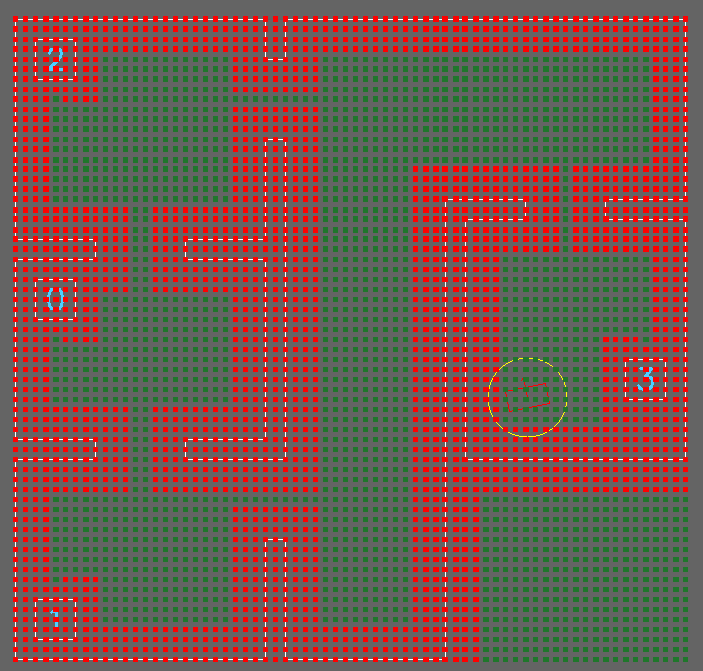
The first step made to build the 2D grid was to break up the world space which was occupied by the hospital environment in equally large pieces. To achieve this, the maximum horizontal and vertical position are saved while loading the corner data from the map file. Then, the grid dimensions were set to the length divided by a grid resolution, which was 0.1 meters as defined in the configuration file, which resulted in a grid with 67x130 cells as seen in figure Xa. In here all the data was set to true as initial value.
The next step was filling the grid with the loaded data stored in the Line2D objects from before. Since these objects stored the beginning and ending of all the walls and side cabinets it was possible to loop over each object, dividing the line between it into smaller segments who could be matched to the grid and setting the corresponding grid cell at the belonging world position to unreachable (false) in the grid. This eventually led to a grid as seen in figure Xb. By giving different offsets to specified Line2D objects it was possible to create some space for error within the movement and path planning, such that PICO will not move directly next to obstructions such as the walls and cabinets. This effect can be seen in figure Xc.
To let PICO react to sensed obstacles within the hospital environment the grid was considered as a living object, which meant that when an object got pushed to the worldmodel that the grid cells corresponding to the pushed object location got put into the grid as unreachable. Just like for the walls and cabinets an offset could be specified which would be filled in the grid around the locations where obstacles were detected. The combined result can be seen in figure Xd
https://github.com/nlohmann/json (opensource json library source link)
http://cstwiki.wtb.tue.nl/images/Mrc2020_finalmap_corrected.zip (provided map json 2020 by TU/e)
http://cstwiki.wtb.tue.nl/images/Finalmap2019.zip (provided map json 2019 by TU/e)
Strategy
The purpose of the strategy class is to compute and return the path that PICO needs to take in order to complete its tasks. This path should be a vector of 2D points in the global reference frame. These waypoints are determined in two steps
First, the shortest path from PICO to its destination is computed using an A* shortest path algorithm. This algorithm is used on the grid nodes of the world map, left figure below. A* is a similar algorithm compared to Dijkstra’s shortest path algorithm. However, due to the implemented heuristic A* is much faster. For a more detailed explanation and/or examples see [1] and [2]. The figure in the middle below shows a path found by the A* algorithm.
After the A* algorithm has found a shortest path, a large vector is obtained with all grid nodes that need to be visited. There is however no need to reach all these points one by one, in fact, using this as a reference trajectory will only slow PICO down due to it correcting for overshoot. For this reason, a string pulling algorithm was used to only keep the waypoints that are strictly necessary in order no not hit any obstacles or walls. This string pulling algorithm works as follows.
It starts evaluating if it can reach the second node from the first node in a straight line without crossing an unreachable space. If so, then it continues evaluating if the third node can be reached and so on. If it stumbles on a node that cannot be reached in a straight line, in other words, it would cross an unreachable grid node on the straight line between the first node and the node that it is being evaluated, then it will save one node prior to the unreachable node and stores this node as a waypoint. The algorithm is then repeated with the saved waypoint as the new node from which the path is evaluated. This process continues until the final waypoint is reached. This results in a vector only containing the waypoints that are strictly necessary for it to reach the target without hitting an obstacle or wall, see the figure on the right below.
Visualization of the grid
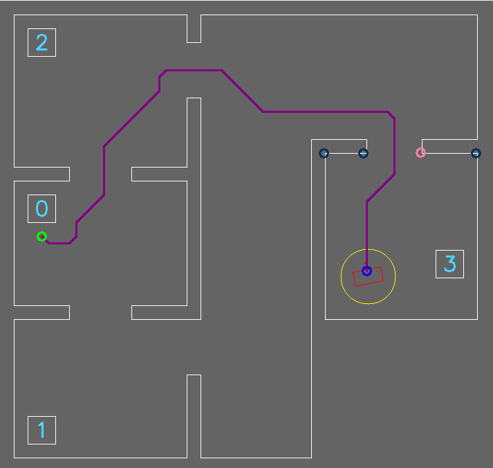
Waypoints
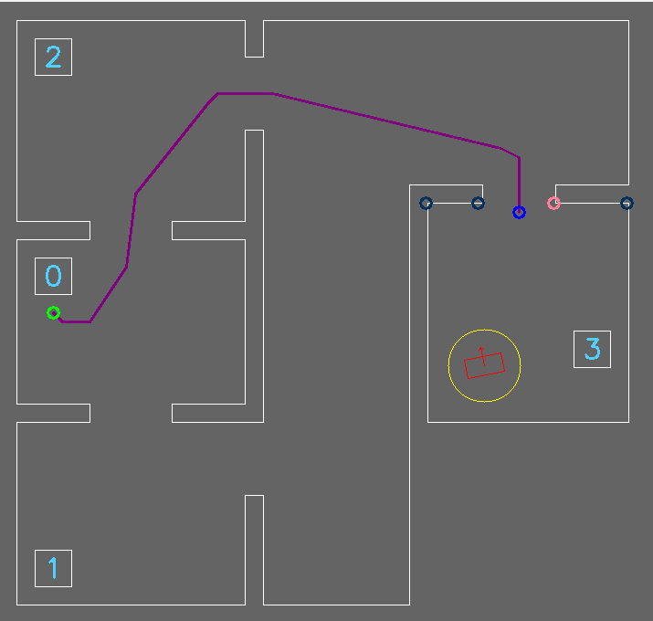
Waypoints with string pulling algorithm


Perception
The main goal of the perception component is to translate the real world data into data which can be used for the simulation. The real world data consists of the LRF-data and the odometry data. Perception uses this data to localize PICO, detect obstacles and to measure the distance to objects around PICO.
Localization
Filtering algrorithm
As explained earlier, perception is able to translate raw LRF data into lines which do or do not correspond with known obstacles from the given simulation map. What this filtering algorithm does is simply checking if the fitted lines are in fact known obstacles, i.e. walls or cabinets, or unknown obstacles. The method of filtering the known from the unknown obstacles is done over multiple procedures which are explained next.
Once the fitted line data is retrieved from the world model, it is converted into a vector containing the coordinates of the first point of the line and the coordinates of the last point of the line. Since these coordinates are local, they first have to be converted to global coordinates. After converting the coordinate system, the actual filtering will take place. This filtering will be done in two steps, namely first filtering out the walls from the fitted lines and last is to filter out the cabinets from the fitted lines. What remains are the fitted lines corresponding to unknown objects, i.e. static or dynamic objects.
The filtering takes place in a specific function. The input for this function consists of one of the fitted lines, to be called F, the data where this fitted line has to be compared with, to be called C, being walls or cabinets, and some thresholds which will be dealt with later on. The output is either a true or a false, since a fitted line does or does not coincide with a certain wall or cabinet.
The first step in comparing a line L to a set of line C’s, is to check whether the normals of the lines have the same direction. This already filters out a large part of the data with a relatively simple, thus saving computation time for later procedures. One of the input margins for this function is the ‘angle threshold’ determining the margin on the difference in the angles of the normal lines. This threshold has been set to a relatively low value, since there cannot be large differences in normal lines for them to be comparable. Comparing normals alone does not suffice. After that step, the distance from the fitted line F to the comparable line C is calculated. This is done by means of a vector projection. This coincides with the z in the figure below.

Specifically the distance from the center of F to C is measured. The reason for this is because in some situations the fitted line data is heavily influenced by noise of the LRF. This mainly occurs when fitting the lines of long hallways. By measuring from the center of F, this problem was solved. Another input threshold for this function is the ‘distance threshold’. This threshold ensures that lines from other parts of the map cannot be compared with the measured line. For instance, the normals from C in room 1 and C in room 2 can coincide with F, but the distance from C in room 1 to F is way smaller than that of C in room 2. Thus the C from room 2 is filtered out.
The final step in comparing line C to a fitted line F is to check whether line F falls within the boundaries of C. This final step is mainly to check if the fitted line F is not a door. In this project it was assumed doors would be somewhat in the center of 2 walls, since in previous years that was the case as well. This however would mean that both the normals would have the same direction and the vector projection would be short, since the distance would be equal to the depth of the door in the wall. This final step filters out these possibilities. The last step checks if the distances from the first and the last point of F to the first and the last point of C are shorter than or equal to the length of C. If so, it means that both points lie in between or on line C. There is a last threshold for this procedure called ‘overshoot threshold’, which ensures that slight differences in distances cannot influence the process. If after all these steps, a line C from the set of comparable lines is left, then line F equals line C and the filtering process for this data set is complete.
This process first compares all fitted lines to all the known walls. The lines that were not comparable to a wall are then compared to cabinets with the same procedure. If there are still fitted lines left after this process, the remaining fitted lines are used to check for obstacles.
Obstacle detection
The obstacle detection process is based on the theory of a histogram filter, but then simplified. The perception of PICO is able to detect obstacles by using the remaining fitted lines after the filtering process. By using a histogram filter it is ensured that not every remaining line is immediately pushed as obstacle. The exact procedure is explained in the following sections.
Once the perception of PICO measures something which is not comparable to either a wall or a cabinet, it is analyzed in the obstacle detection function. The first time something enters this function, the line data, combined with an initial weight of 1, is saved in an array. If the next loop of the main cycle, another line enters the obstacle detection function. This new fitted line is compared to the line which is saved earlier. By means of the filtering algorithm described before, the new fitted line is either similar or not similar to the earlier saved line. Which leads to two different scenarios. If the new fitted line is similar to the earlier saved line, it means the same line is measured twice. In this case, the weight of this line in the array is increased by 1. If the two lines are not similar, the new fitted line will be added to the array of earlier measured lines with a weight of 1 and the earlier measured line will have a weight decrease of 0.5. This procedure repeats itself every new cycle of the main loop. Once a certain line has a weight of 0 or lower, the line is deleted from the array of earlier measured lines meaning it was probably a wrong measurement. If a line has a weight which is bigger or equal to the number specifying the rate of the main loop, that line is pushed to the world model as an obstacle. The world model ensures this data is processed accordingly.
Potential field
The potential field enables PICO to safely move in any direction. It measures distances from itself to objects and finds the direction in which moving can be done safely. The potential field is designed in the following way.
After obtaining a trajectory from the strategy/planning component, PICO starts moving in the desired direction. This desired direction can be visualized by a vector pointing towards the next waypoint. As mentioned before, the potential field measures the distances from PICO itself to objects around it. The potential field is specified to be around 30 centimeters around PICO itself, ensuring that objects far away will not have any influence on the movement. Thus, as long as objects are out of the range of the potential field, the potential field will not give any direction since the sum of all vectors in the potential field will result in 0. This will on its turn result in a movement in only the direction of the desired direction. This can be seen in the most left figure of the figure below.
Once an object (or objects) enter(s) the potential field, the vectors in the potential field will have different lengths. This will result in a potential field vector pointing in the direction where the distances to any object are equal. Adding this vector to the desired direction vector results in the right figures of the figure below. Once the sum of all the potential field vectors equals zero again, the direction will again be decided by the desired direction vector.

To ensure the ‘power’ of the potential field vector will not dominate the ‘power’ of the desired direction vector or the other way around, both vectors are scaled to perform optimally.
Line fitting
.
Movement
The purpose of the movement class is to compute and send reference velocities to PICO’s actuators. It uses both the potential field from the perception class as the next target node coming from the computed path from the strategy class to determine its direction.
First, the potential field and the target are converted to two unit vectors pointing in the desired directions for each. These vectors are then scaled according to the “obstaclePriority” variable. This value determines how much PICO should focus on avoiding obstacles instead of following its target. An obstacle priority of 1 results in PICO purely driving on the potential field whereas an obstacle priority of 0 results in PICO blindly following the target direction. After testing, an obstacle priority of 0.5 gave the best results. After scaling, the target and potential field vector are added up to find the movement vector. This vector determines the direction in which PICO should move
Next, the angle and distance to the target point are computed. Once these computations are done, three proportional controllers are used to compute the three reference velocities. This is done in the following manner.
First, a proportional controller is used to rotate PICO towards its target where the input to the controller is the difference between PICO’s target angle and its own orientation. Once PICO is within a certain margin of its target it uses two more proportional controllers to compute the velocities in its x and y frame. This time, the movement vector is used together with the distance to the target as an input to the controllers. It has to be noted that the computed velocities are saturated to remain within the maximum allowed velocities.
When a path node is reached (with a certain margin) PICO will send a Boolean signaling it has arrived at the target. Note that this margin is larger for the path nodes compared to the last node in the path (cabinet node). This is done since PICO does not need to track the reference perfectly, however, it needs to be at the precise location when arriving at the cabinet. Also, when arrived at the cabinet, the movement class will align PICO to the cabinet using the same proportional controller as for the rotation in the moving algorithm.
Monitoring
The monitor class serves as a safety net in case PICO shows undesired behavior. Initially the monitoring checked multiple cases. First of all, if an object was too close to PICO a flag would be given. The object would be in PICO’s safe space which is a circle around PICO with a certain radius. Furthermore, if the potential field vector became too large, also a flag would be given. The idea was that if the potential field vector became too large, PICO should not be able to pass an object. Lastly, if something was placed on the desired location of PICO, also a flag would be given. There was initially thought that in this case the path of PICO could not be continued. However, since the desired locations of PICO is reached by means of waypoints, the waypoints could be changed in order to reach the desired location.
Eventually, only the following flag is used in the hospital challenge. The grid that is used consists of nodes which are accessible or not. A node is not accessible if an object is located on it. If a node that is used in the A* path planning coincides with an inaccessible node, a flag will be given. Because all relevant obstacles were acknowledged by the grid, PICO creates a new path when his previous path is blocked by an obstacle.
The first two flags were not used because the parameters of the potential field are chosen in such a way that these flags would not become true. A snipped of the c++ code of the monitor class is showed in this link...
Visualization
Hospital Challenge result
In general, the Hospital Challenge showed to be a success. The initial localization was completed almost instantly and was maintained for the biggest part of the challenge. The histogram filter detected the static obstacles rather well and the potential field dealt with the dynamic obstacles as intended. It also prevented some crashes when the localization was lost. There were however also some problems which together resulted in a DNF.
Firstly, during testing, doors were interpreted as a single line within a doorway instead of the doors being completely flush with the walls. This resulted in a rather slow detection of the doors since the detection of the doors (and objects) is mainly based on finding the corners of the objects/doors. Even though not instantly detected, PICO eventually would realize there was a closed door in front of him updating his path to its target. *if possible, insert gif of Pico in front of door*
The second problem occurring was a due to an error in its localization. The first attempt resulted in a DNF due to bad localization. This occurred in the room of cabinet 6 and was caused by an offset in PICO’s localization. When PICO reached the cabinet it thought it had to move a bit further due to an offset in his localization. This resulted in PICO’s strategy telling him to drive forward but the potential field telling him to drive backward, this together caused a deadlock and hence the attempt was stopped. *if possible, insert gif of offset in room 6*
The second attempt also failed, this time in the room with cabinet 1. PICO’s frame would occasionally rotate and thus give a false positive of an object in the grid, obstructing its path. A monitoring function was implemented to deal with these kind of scenarios. When no path can be found to PICO’s target this means that a false positive has occurred somewhere. This monitoring function would then raise a flag to clear the grid of all detected obstacles which allowed PICO to find another path. However, in the hospital challenge, PICO would keep getting false positives due to bad localization resulting in an infinite loop of resetting the grid and finding no path. *if possible, insert gif of this infinite loop*
The bad localization had two reasons. Firstly, the localization is based on detecting features in the map (e.g. corners). However in the hospital challenge objects were added that “cluttered” these features. Secondly, since the doors were closed flush with the walls, two additional corners could not be used to localize PICO and together with the objects this seemed too much to handle in the room with cabinet 1.
Even though PICO did not finish its objective, we became second place. This was due to PICO not crashing and driving safely at all times. Also, it was believed that given more time PICO would eventually get a better localization and being able to finish.
To summarize, all functionalities of PICO performed well with the exception of the localization and door detection. These should be improved in the future.
Discussion
- What went wrong and why? - What would we do differently next time? - Were our choices good and why?