Embedded Motion Control 2014 Group 5

Group 5

Name	Student	Email
Paul Blatter	0825425	p dot blatter at student dot tue dot nl
Kevin van Doremalen	0797642	k dot p dot j dot v dot doremalen at student dot tue dot nl
Robin Franssen	0760374	r dot h dot m dot franssen at student dot tue dot nl
Geert van Kollenburg	0825558	g dot o dot m dot v dot kollenburg at student dot tue dot nl
Niek Wolma	0633710	n dot a dot wolma at student dot tue dot nl

Planning

Week 1 (21/4 - 25/4)

- Instal Ubuntu
- Instal ROS
- Setup SVN
- Tutorials

Week 2 (28/4 - 2/5)

- Continu tutorials
- Setting up program for first test

Week 3 (5/5 - 9/5)

- Finishing tutorials
- Continu on program first test
- First test robot
- Program architecture: File:Nodeoverview.pdf

Week 4 (12/5 - 16/5)

- Everyone has finished the tutorials
- Working on program for the robot (we started too complex and therefore we have to build a more simple program for the corridor challenge)
- Setting up program for corridor challenge
- Second test robot (unfortunately, we didn't manage to test with the robot)
- Corridor challenge (PICO did the job with our program, which wasn't tested before! More information about the program can be found below.)

Week 5 (19/5 - 23/5)

- Meeting with tutor on Tuesday May 19th
Update of the current status with the tutor. There are no problems at the moment. We will keep working on the program for the maze challenge.

The following subjects will be discussed during the meeting:
- Evaluation corridor challenge
- Setting up a clear program structure (group): File:EMC05 scheme pdf.pdf

- Possibilities and implementation of odometry data (Geert)
- ROS structure (Robin)
- Improvement of program for corridor challenge for implementation in final challenge (to be defined)
- Review literature path planning (Geert)
- Detection of arrows with camera (Robin/Kevin)
- Situation detection (Paul/Niek)
- Finishing wiki corridor competition (Geert)

Week 6 (26/5 - 30/5)

- Odometry (Geert)
- Arrow detection (Kevin)
- Drive node (Paul)
- Intersection detection (Niek)
- ROS structure (Robin)

Week 7 (2/6 - 6/6)

- Arrow detection (Kevin)
- Drive node (Paul/Geert)
- Intersection detection (Niek)
- ROS structure (Robin)
- Setting up presentation (Kevin)

Week 8 (9/6 - 13/6)

Continu to work on:
- Intersection node (Niek/Robin)
- Drive node (Paul/Geert)
- presentation (Kevin)
- Add averaging to arrow node (Kevin)
- Update wiki (Kevin)

June 13th: Presentation strategy and program (all student groups)

Week 9 (16/6 - 20/6)

June 20th: Maze challenge with PICO (all student groups)

Introduction

The goal of this course is to implement (embedded) software design (with C++ and ROS) to let a humanoid robot navigate autonomously. The humanoid robot PICO is programmed to find its way through a maze, without user intervention. On this wiki page the approach, program design choices and chosen strategies which are made by group 5 are presented and explained.

Corridor Challenge

The corridor challenge was on Friday May 16th 2014. In the days before the corridor challenge the program was build and simulations were run with Gazebo. Due to some implementation errors and programming difficulties, the program wasn't tested in real on PICO before the challenge. However, with this program PICO managed to finish the corridor challenge! The strategy of the corridor challenge will be explained with the following pictures and further improvements will be considered.

First, an aligning function is added to the program. PICO has to drive through a corridor without hitting the wall. The aligning function compares the distance to the wall of the laser angle of -180 degree and +180 degree w.r.t. to the x-axis of PICO. When the difference between these distances becomes to large, the program sends a rotation velocity to PICO in a way that this difference will be decreased up to a certain threshold. With this aligning function PICO will be kept in the middle of the corridor. Second, the corner detection looks at two laser points at the left and two laser points at the right side. The laser points at each side have a different angle (difference around 2.5 degree).

A corner is detected when the difference between the laser points at one side (right or left) is above a certain threshold (=1.0 meter). Then the aligning function and corner detection function stop and the program starts with the cornering function. The cornering function detects directly the smallest distance (R) on the y-axis of PICO with respect to the wall in the corridor. The angular velocity and y-velocity are set in the program to keep the minimum distance r at the y-axis of PICO and to keep this distance equal to R. With this strategy PICO can drive through a corner and after the corner PICO is almost directly aligned with the next corridor. This finalizes the explanation of the program which is used in the corridor challenge.

Further improvements followed from the corridor challenge are:
- Implementation of odometry data which can solve the problem that PICO didn't correctly turn 90 degrees in a corner (corridor challenge).
- Use of laser range instead of some laser points.
- Calculation of thresholds and possibility of variable thresholds.

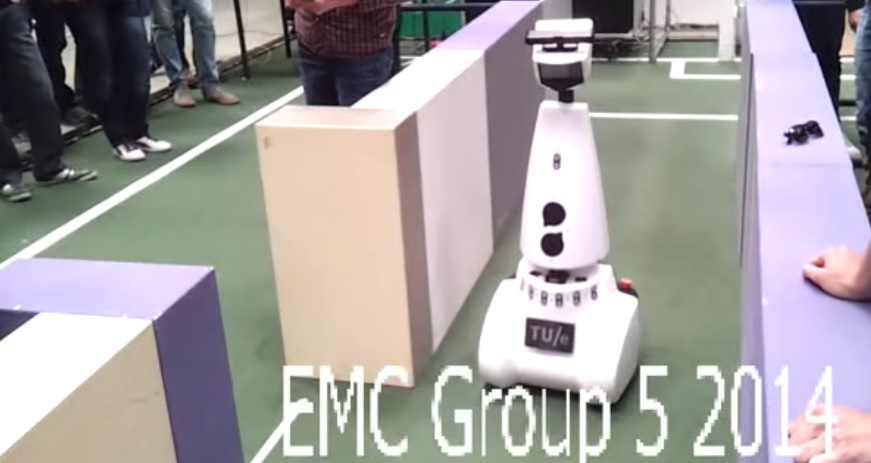
Movie corridor challenge

Below a movie of PICO during the corridor challenge:

Maze Challenge

The maze challenge is an extension of the corridor challenge, which will take place on the [math]\displaystyle{ 27^{th} }[/math] of June.

Solving strategy

The wall follower is one of the best known maze solving strategies. If for the maze all walls are connected together and there is only one exit in the maze (and the maze does not contain loops), than following the wall on your left or right hand side will lead you always to the exit [1]. An example of solving a maze using the right hand side wall follower strategy is depicted here below.

There are many other maze solving algorithms (depth-first-search, pledge, Trémaux), but since we don't know anything about the maze à priori, we will make use of the left hand side rule of the wall follower strategy.

Program Architecture

The implemented program architecture is as depicted in the Figure below. We will make use of four different nodes, namely; "drive", "decision", "arrow detection" and "situation detection". The drive node uses odometry and laser data, the arrow detection node uses camera data and the intersection detection node uses laser data. The arrow and intersection detection node will send messages to the decision node, which decides whether PICO has to go left, right, straight or has to rotate 180 degrees. The decision node will send its decision information to the drive node, and the drive node will respond on this information.

Laser data

The LFR (Laser Range Finder) is Pico’s primary source of orientation. Approaching intersections are detected and analysed using the laser range data. The situation detection node uses the laser data as input to map its surroundings, and publishes the found pathways for the decision node.
A typical laser data message contains an array of approximately 1080 points with the corresponding distances w.r.t. Pico. This gives Pico a 270 degree wide and 30 meter deep field of vision. An example of a scan is depicted below.

Odometry

Odometry is the use of data of the angular positions of the robot wheels. This data is used to estimate the position of the robot relative to a starting point. The angular positions are converted into Carthesian coordinates (x-, y- and theta-direction), where
[math]\displaystyle{ \theta = tan^{-1} \left( \frac{y_{1} - y_{2}}{x_{1} - x_{2}} \right) }[/math]
This data is never fully accurate, inter alia due to wheel slip. The angle is reset when the rotation of the robot is completed.

Situation detection

Using a polar to cartesian conversion, the data can be plotted in the [math]\displaystyle{ x,y }[/math] plane. In the picture below the robot is located at the point (0,0) and is standing in a skewed orientation in an approx. 1 m wide passage. The passage itself is a dead end, but there clearly is a possible exit on the right side of the passage (indicated by the green arrow).

The situation detection node scans the data for ‘jumps’ in the distances between sequential data points. E.g. the point with index 525 clearly has a larger absolute distance to the origin than the previous point (not labelled). Scanning the data for these jumps at orientations [math]\displaystyle{ 0 \pi - 0.25 \pi }[/math] and [math]\displaystyle{ 0.75 \pi - \pi }[/math] will indicate upcoming pathways on the right and left side of the robot respectively. When a possible pathway to the left or right is detected the node looks at the data points around [math]\displaystyle{ 0.5 \pi }[/math] and determines whether the current pathway continues or comes to an end. Three Booleans named Left, Straight, Right are published according to the found results.

In order to increase the robustness of the situation detection algorithm and the accuracy of the prediction, the node examines several points around the found jumps to filter out measurement errors or errors in the actual maze (a small hole in the maze would be interpretted as a jump but doesn't qualify as a passage).

Furthermore the situation detection node scans for dead ends in the range [math]\displaystyle{ 0 \pi - \pi }[/math]. In this specified range the node calculates the cartesian distance between all sequential points. If no wide enough passages are detected a Boolean called Deadend is set to 1. This signals the decision node to turn around immediately. The deadend detection function also uses averaging to increase robustness.

The situation detection node thus publishes a total of 4 Booleans, named Left, Straight, Right and Deadend.

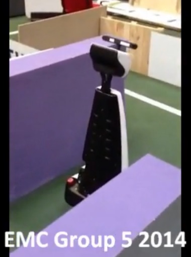
Movie dead-end detection

Below a movie of PICO during testing dead-end detection:

Arrow Detection

Step 1: HSV image[2]
The camera image from the PICO (RGB image) is converted into an HSV (Hue, Saturation, Value) image, which is a cylindrical-coordinate representation of an RGB image. Hence, one can set a hue (tinge), saturation (intensity) and value (luminance/brightness) instead of red, green and blue values. The values for the image are represented by a colour wheel, which starts and ends with the colour red. Since the arrow will be red coloured, two HSV image representations will be merged to get a nice image of the arrow.

Step 2: Blurred image and edge detection
Firstly, a binary image is created (by setting thresholds) wherein red coloured objects will appear as white and all other colours will appear black as depicted on the left hand side in the Figure below. Secondly, the image is blurred (noise is filtered out) by setting a kernelsize, which denotes the range (fixed array size) along an anchor point. Than edges (which are jumps in intensity) are detected by setting a threshold and using the Canny edge detector algorithm [3] [4]. The image of the edge detection is shown in the middle of the Figure depicted below.

Step 3: Hough transform[5]
A Hough transform is done to detect straight lines in the image by using the slope-intercept model. Straight lines can be described as [math]\displaystyle{ y = mx + b }[/math], where [math]\displaystyle{ m }[/math] denotes the slope and [math]\displaystyle{ b }[/math] the [math]\displaystyle{ y }[/math]-intercept. For an arbitrary point on the image plane ([math]\displaystyle{ x }[/math],[math]\displaystyle{ y }[/math]), the lines that go through that point are the pairs ([math]\displaystyle{ r }[/math],[math]\displaystyle{ \theta }[/math]) with
[math]\displaystyle{ r(\theta) = xcos(\theta) + ysin(\theta)~~\forall~~r_{\theta} \gt 0,~~0 \lt \theta \leq 2\pi }[/math].
At last the detected lines are drawn on the RGB image as shown on the right hand side in the Figure below.

Step 4: Direction detection
The direction of the arrow is detected by calculating the gradient of the lines detected with the Hough transform. The gradient is calculated by
[math]\displaystyle{ \nabla = \frac{y_{1} - y_{2}}{x_{1} - x_{2}} }[/math]
When the gradient is positive it denotes a line going downwards, a negative gradient denotes a line going upwards. By determining which line is above the other one, we can determine the direction.

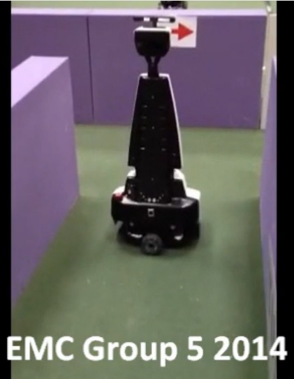
Movie arrow detection

Below a movie of PICO during testing the arrow detection. As desribed before, PICO will automatically turn left, but now the arrow will overrule the left hand rule.

Decision

Decision uses information from the arrow and intersection detection to give commands to the drive node. Using the left hand rule in combination with arrow and dead end detection results in the following hierarchical structure:
-arrow (if detected)
-dead end (if detected)
-left
-straight
-right

The arrow detection is used on T-junctions to overrule the left hand rule and turn right if the arrow points in this direction.

Drive

The drive node will execute the commands it receives from the decision node. Furthermore the drive node includes an aligning function to keep the robot driving in a straigt fashion, a safety function to prevent collisions and a recovery function in case the safety function has been triggered.

Crossing intersections

Alignment

Safety

Recovery