Embedded Motion Control 2014 Group 10

Members of group 10

Bas Houben	0651942
Marouschka Majoor	0660462
Eric de Mooij	0734166
Nico de Mooij	0716343

Planning

Week 1

• Introduction
• Install Ubuntu

Week 2

• Determine the course goals
• Brainstorm about the robot control architecture
• Start with the tutorials

Week 3

• Continue with the tutorials
• Install ROS/QT
• Finish robot control architecture
• Brainstorm about collision principle
• Brainstorm about navigation

Week 4

• Meet with the tutor
• Finish installation
• Finish tutorials
• Write collision detection
• Write corridor navigation
• Test the written code on Pico
• Corridor challenge (Recorded performance)

Concepts

Robot program architecture

While the initial idea was to give every distinguishable function its own node, only a few functions have been given their own node. This has been done because several functions have to communicate large matrices with each other, making global variables the superior option. Besides the laser, camera and drive node's provided by the course, we added two additional nodes: the image recognition node and the navigation node.

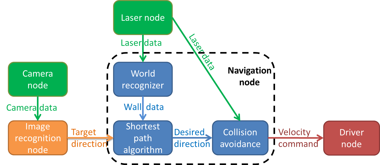
The decision making of pico consists of 3 main steps, listed below

Determining strategy

In the first step, pico determines what strategy to apply, depending on whether an arrow is detected or not. The default strategy is to follow the wall to the right, executed by taking every right turn available. However, when an arrow is detected in the distance, the strategy is changed to driving straight forward, towards the arrow. If the arrow is close enough to take the turn, the strategy is set to either the right hand rule or left hand rule, according to the direction of the arrow. When no arrow is detected, the strategy will return to the default right hand rule. This step involves the 'Camera node' and the 'Image recognition node', which will be explained in more detail later. The 'Camera node' sends camera data to the 'Image recognition node', which then searches for an arrow. The image recognition node provides a target direction for the second step, according to any arrows it might recognize.

Path finding

In the second step, the strategy determined by step one will be executed with the aid of Dijkstra's shortest path algorithm. This algorithm detects whether a turn is available, and whether it has a dead end or not. It then calculates a desired direction according to the turn options available. This step involves the 'Laser node' and the 'World recognizer" and 'Shortest path algorithm' functions of the 'navigation node'. These two functions will be explained in further detail later on. The 'Laser node' sends laser data to the 'World recognizer' function, which makes a map of the walls currently visible, and stores it in a matrix. The 'Shortest path algorithm' function uses this matrix to determine a desired direction, which is used in the third step.

Collision avoidance

In the third step, the desired direction provided by the previous step is checked for collisions, and altered accordingly. This involves the 'Laser node' and the 'Collision avoidance' function of the 'Navigation node'. The 'Laser node' provides the 'Collision avoidance' function with laser data. This data is used to determine if any walls come within a certain safety range. When this occurs, the desired direction provided by the previous step is altered to avoid collisions. If no collisions are imminent, the desired direction is left unaltered. The possibly altered desired direction is transformed to a velocity command, which is then send to the 'Driver node'.

Robot program architecture

The idea of our architecture is to create different process layers. By splitting the incoming signals and combining them later, the tasks can be divided and the different processes can run in parallel. Layers are based on the available sensors as much as possible.

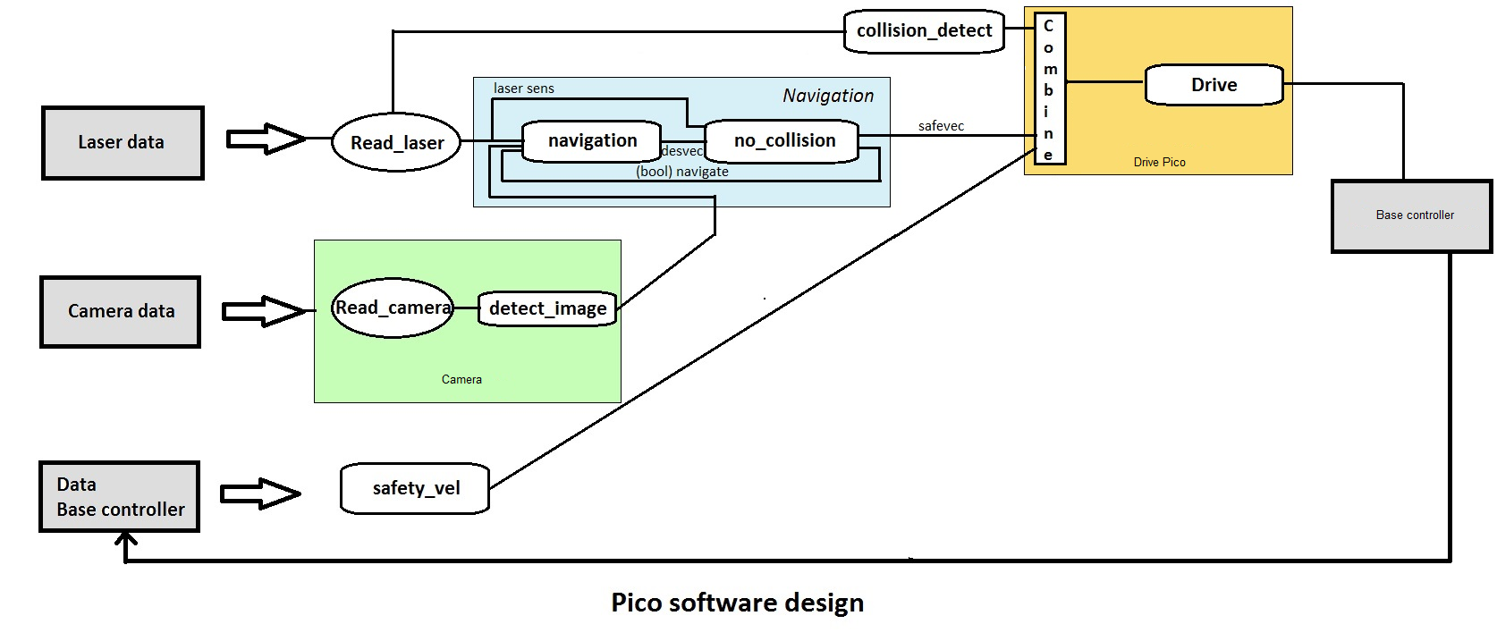
Wall detector

The wall detector determines whether the robot is close to a wall or not by determining the unblocked distances at its two sides. When either side is too close (within 30cm) it turns parallel to that side, taking a distance of 30cm from the wall.

Intersection detection

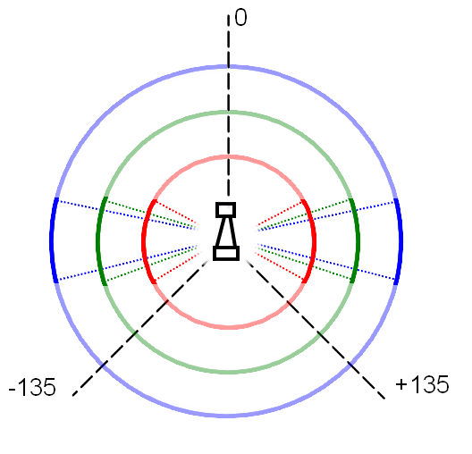
When driving forward, Pico uses the measured distances at different angles from the laser data in order to detect corridors. These distances are visualized in the figure on the left. The red circle part covers 72 degree with a radius of 0.5m, the green circle part covers 35 degree with a radius of 1.0m and the blue circle part covers 25 degree and a distance of 1.5m. The circle part tips outside of pico are on two parallel lines 60cm apart. When each of this circle parts doesn't detect any obstacles inside, this is considered to be the corridor.

All holes smaller than 0.30m will never be detected as corridor because the slimmest part of the laser range bundle outside pico is 0.30m. (Just outside the part covered by the red circle part, inside the blue circle part). The smallest hole that always will be determined as corridor is 0.60m; the laser covers a with of 0.6m. Holes within 0.30m and 0.60m might be determined as corridor, dependent on the length of the exit and pico's positioning.

Intersection determination

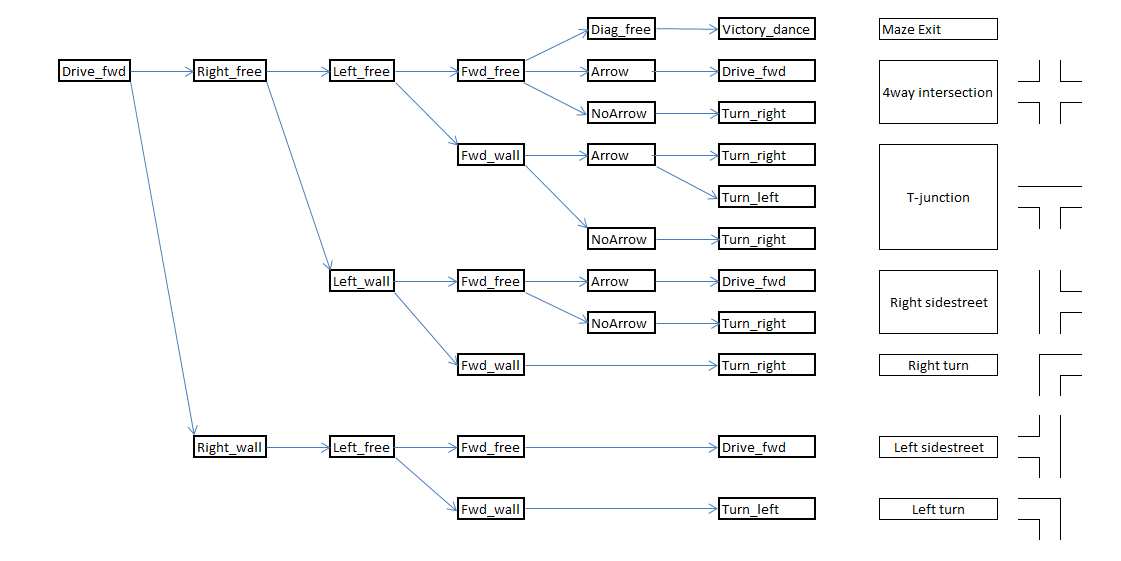
Depending on the results from the intersection detection part, Pico will determine which situation he is in. In the maze, these situations could be 4-way intersection, corners and T-junctions. The image below shows how each situation is determined depending on the presence of a wall or corridor in the forward, left or right detectors. At this point, arrows can not yet be detected, so that part of the protocol is skipped. Once arrow recognition is implemented, the arrows will be used to determine the correct corridor to take at T-junctions, or to move towards a T-junction at the end of a corridor, if an arrow is detected in the distance.

Moving through intersections and corners

Once Pico has detected a situation and determined if he want to turn, he will rotate + or - 90 degrees. After the rotation, Pico will drive forward a small distance to position himself fully into the next corridor and will look around once more.

Arrow Detection

To recognize or a given arrow is pointed to the left or to the right, and to let Pico react on this, several steps are followed while driving Pico:

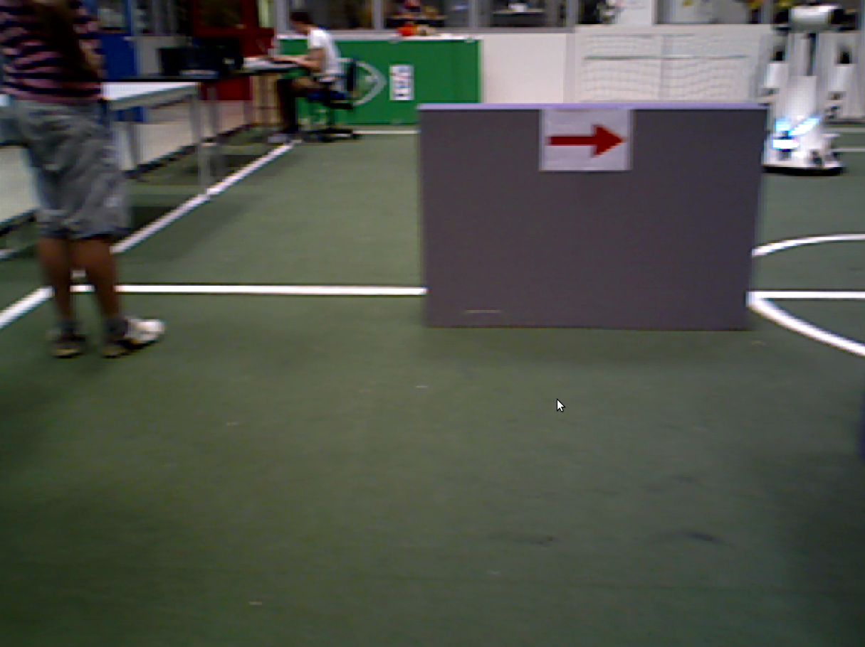
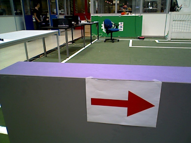
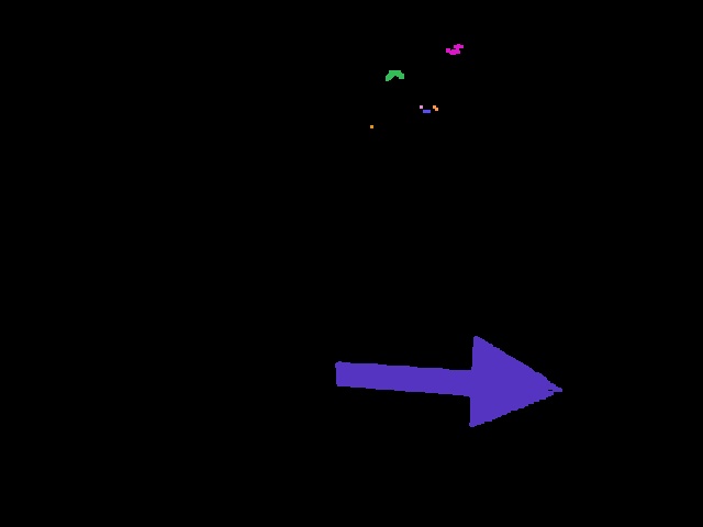
Step 1: The ROS image is converted to an Open CV image. Picture used as example:

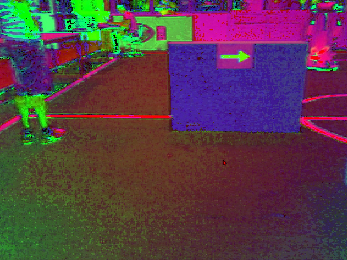
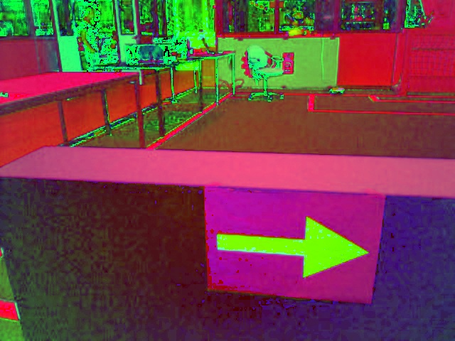
Step 2: There are different color spaces to describe pictures. In our case the RGB image is converted to an HSV image. HSV is commonly used in computer based graphic design. Converting RGB to HSV and vice versa is unambiguous. This results in the following picture:

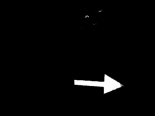
Step 3: The red pixels are filtered out, in other words the HSV image is tresholded which results in a binary image. The tresholded picture looks as follows:

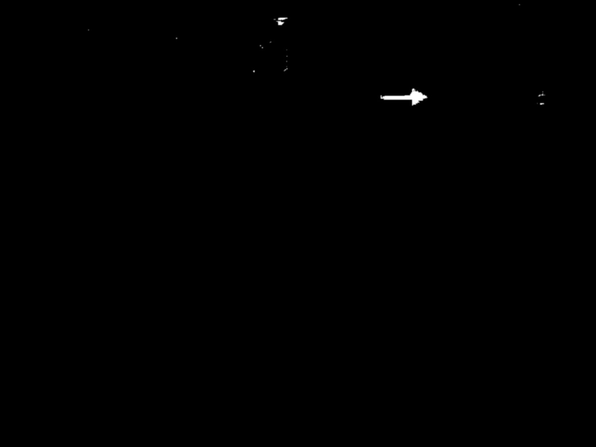
Step 4: The binary image gives the different red spots a little bit frayed contours. Therefore the image is blurred, in other words the contours are smoothened and some pixels are filled up to create a fully padded area. This is done with the floodfill algorithm, which works a bit like a minesweeper game. This results in the following picture:

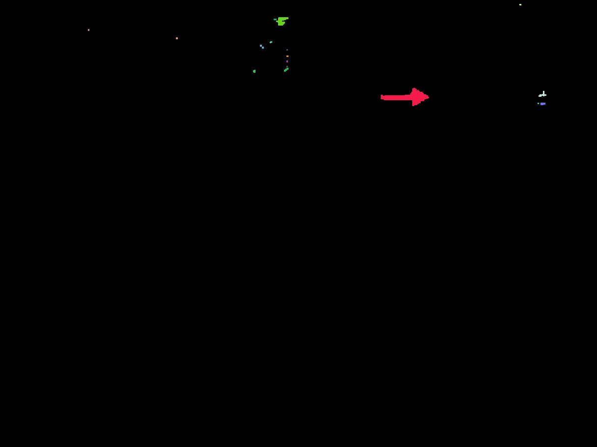
Step 5: With the OpenCV option findcontours the different contours of all the red blobs are found. For each founded contour, the corresponding blob is coloured differently. This results in the following picture:

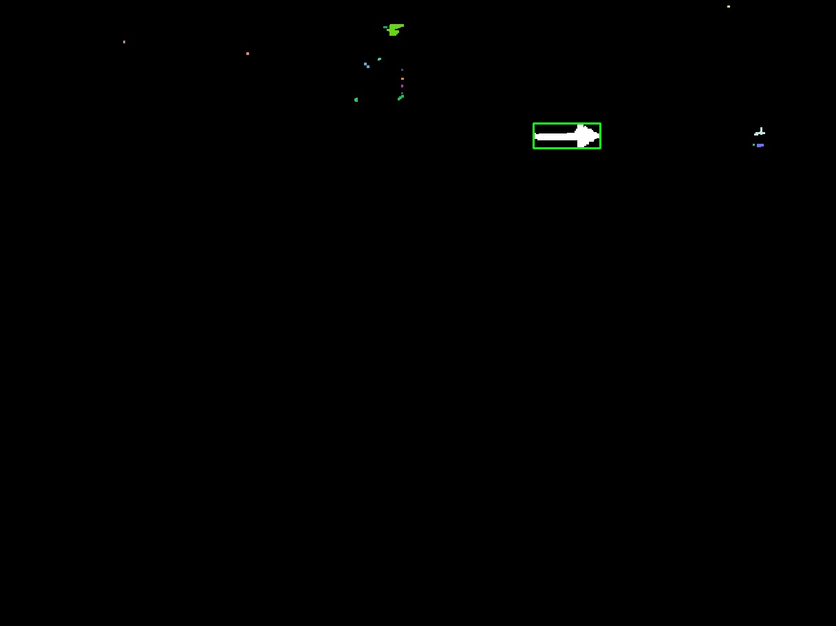
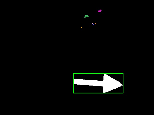
Step 6: Now the areas inside all different contours are calculated. With a loop the largest area is determined. The largest area is assumed to be the arrow. (Important assumption, because a other large red area which is larger than the area of the arrow may let the arrow recognition fail). When the largest area is found, a closest rectangle is drown around the area. This results in the following picture:

Step 7: The largest area counts the number of dots of the arrow. A minimum number of dots is set, to determine if an possible arrow can be recognized.

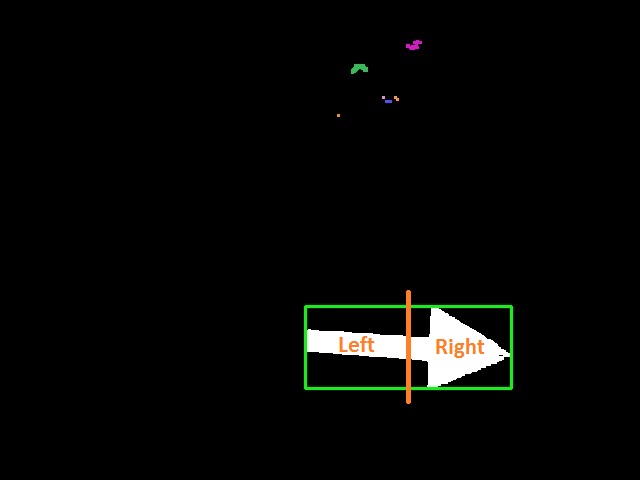
Step 8: The rectangle is now divided in two equal parts, a left and a right part. This is done by creating two different ROI’s (Regions of interest) on base of the coordinates of the rectangle. This can be visualised as follows:

Step 9: This is the last step where the direction of the arrow is recognized. The number of red dots are calculated for the left part as well as the right part. The arrow is pointed to the sight with the most red dots.

Step 10: Once the arrow is detected and its direction is verified, the main node must be told. This is done by sending an integer over a ROS-topic:

0: No arrow detected

1: Small (faraway) arrow detected

2: Large (near) left arrow detected

3: Large (near) right arrow detected

World recognizer

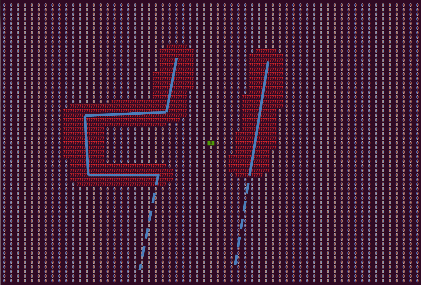
The 'World recognizer' function converts the laser data provided by the 'Laser node' to a matrix used in the 'Shortest path algorithm' function. This matrix contains all areas pico is not allowed to go. The matrix represents a square grid around pico. The amount of cells and cell size are determined before hand. A zero in the matrix means that the respective cell is unoccupied. Each point of the laser data array is transformed to a position in the grid, and every cell in a safety circle with a diameter of 5 cells around this point are marked as occupied. Walls get the number 777 assigned to their cells. Assigning walls with a distinct number allows for easier reading. The safety circle is added to maintain a distance between the walls and the optimal path. In the picture below, an example of the matrix with detected walls is shown.

The walls are represented by the blue line's which are dotted for walls outside pico's vision range. The occupied matrix cells are depicted by the number 777, colored red. The 0 with the green rectangle is the position of pico. As can be seen, angle's of 90 degree are not depicted as such, which can be caused by inaccurate laser data, scaling errors, or inaccuracies in the laser range detectors specifications. However, slight curving of walls does not in navigational errors, and is thus of little importance.

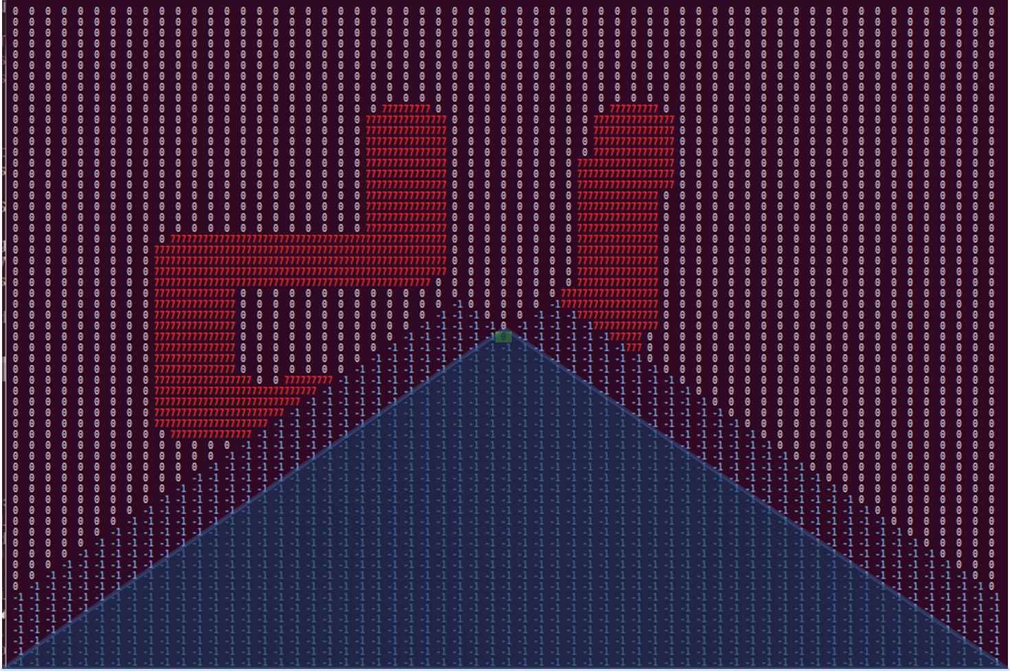
To prevent pico from driving to his blind spot, all non visible cells are marked as occupied, this time with the number -1. Again, a distinct number for each kind of occupation allows for easier reading and coloring of the matrix. The physical blind spot is expanded by a region on each side, to prevent pico from turning back into the corridor he came from. These artificial blind spots have the added benefit of initiating a deadlock when pico is driving head first into a wall. How this deadlock works is explained in the section about the optimal path algorithm. In the image below, the matrix is shown with blind spots.

Again, the red numbers 777 indicate that a grid is occupied by a wall, and the 0 with green rectangle is pico's position. In addition, each blue -1 represents a cell in the blind spot.

Shortest path algorithm

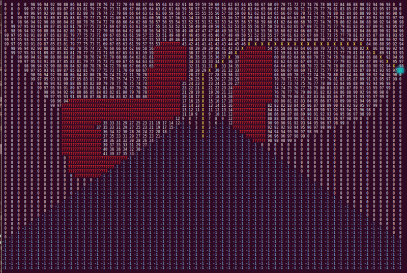
The matrix provided by the 'World recognizer' function is used in the 'Shortest path algorithm' function to determine the optimal path with the use of a modified version of Dijkstra's algorithm. The algorithm starts at pico's position, and looks if the adjacent cells, including diagonal ones, are occupied. In the grid matrix, every adjacent cell with a zero will be occupied, changing the zero for a cost number. The cost number is dependent on how long the path it belongs to is. The shortest path available, thus with the lowest cost number, is the first to be expanded. A horizontal or vertical move adds a cost of two, and a diagonal move a cost of 3. The expansion of paths is looped until the target point is encountered. The target point is represented by a 999 in the matrix, and is placed either above pico, to the right and slightly above, or to the left and slightly above, depending on which target direction has been received from the 'Image recognition node'. In the image below, a the matrix containing the walls and blind spots is depicted after the path finding algorithm.

In this image, the red 777's are again the walls, the blue -1's are the blind spots, the 999 is the target point, in this case for the right hand rule, and the white numbers are the pathing costs. The yellow crosses represent the optimal path.

The pathing algorithm has some additional features. The most important one is the already mentioned deadlock. When no optimal path can be found for two consecutive iterations , pico initializes a 90 degree turn in the opposite direction of the target point. This does also occur when pico gets stuck. Furthermore, the walls are inflated, as mentioned before, which means that small gaps are not seen as corridors. The path finding algorithm runs twice per second, and outputs a desired direction vector, which is the vector describing the distance between the 5th pathing point and the first pathing point, which is located at pico's position. This point should represent the direction pico should drive to follow the beginning of the path. The fifth point is chosen because it is a nice compromise between the advantages of the first few points and points further down the path. Points close by have a very large angle increments, for example 45 degrees for the second layer. Points further down the path run the risk of ending up at the other side of walls, in case the path wraps around a wall. Since walls are at least 5 cells wide, this is not possible with the 5th point.

Path Planning

The intersection based navigation system only works for perfect situations. In order to make the navigation more robust and able to tackle more complicated situations, a shortest path finding algorithm is implemented.

Wall detection and representation

The navigation algorithm uses a matrix to represent the local area around Pico. Collect laser data is placed inside this matrix. The detected walls are inflated to make sure that Pico does not recognize small openings between wall sections. The inflation layer is also used to give the planned path a certain distance parallel to the wall.

Target point location

Pico will be provided with three possible target points: Straight ahead, upper left or upper right. If no arrow is detected, the primary direction places the target point left or right. The arrow recognition will communicate if an arrow is detected. If an arrow is seen in the distance, the target is set to straight ahead. If Pico is close enough to an arrow, the arrow determines the target point location.

Shortest path algorithm

The empty cells in the matrix are now filled with numbers that correspond to the cost (in terms of distance) of driving to that cell. Using Dijkstra's algorithm, the cheapest path is selected. The found path is used to determine the direction vector.

The process is repeated with a frequency of 2 Hz.

Addition of blind spot

As Pico is going around a corner, the old corridor might be seen as the shortest path. To prevent this, an artificial blind spot is added behind and slighty left- and right-behind Pico to prevent Pico from turning back into the previous corridor.

Path planning matrix example

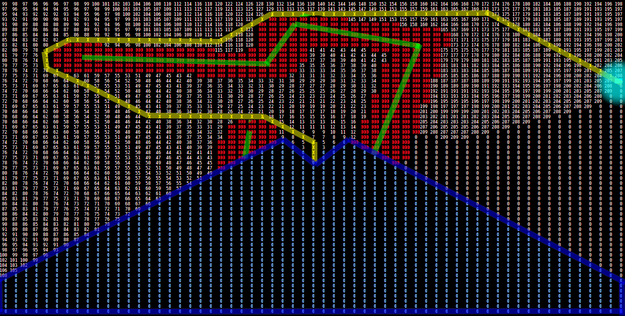
Below is an image representing the matrix during the path planning stage.

-Green: detected walls

-Red: inflated walls

-Blue: blind spot

-Light Blue: target

-Yellow: shortest path

-White numbers: path cost