Embedded Motion Control 2013 Group 5

Group members

Name:	Student ID:
Arjen Hamers	0792836
Erwin Hoogers	0714950
Ties Janssen	0607344
Tim Verdonschot	0715838
Rob Zwitserlood	0654389

Tutor:
Sjoerd van den Dries

Planning

Weekly meetings

DAY	TIME	PLACE	WHAT
Monday	11:00	OGO 1	Tutor Meeting
Monday	12:00	OGO 1	Group meeting
Friday	11:00	GEM-Z 3A08	Testing

Deadlines

DATE	TIME	WHAT
September, 25th	10:45	Corridor competition
October, 23th	10:45	Final competition
October, 27th	23:59	Finish wiki
October, 27th	23:59	Finish peer review

Figure 2: Line detection OpenCV

Progress

Week 1:

• Installed the software

Week 2:

• Did tutorials for ROS and the Jazz simulator
• Get familiar to 'safe_drive.cpp' and use this as base for our program
• Defined coordinate system for PICO (see Figure 1)

Week 3:

• Played with the Pico in the Jazz simulator by adding code to safe_drive.cpp
• Translated the laser data to a 2d plot
• Implemented OpenCV
• Used the Hough transform to detect lines in the laser data
• Tested the line detection method mentioned above in the simulation (see Figure 2)
• Started coding for driving straight through a corridor (drive straight node)
• Started coding for turning (turn node)

Week 4:

• Reorganize our software architecture after the corridor competition
• Created structure of communicating nodes (see Figure 3)
• Finish drive straight node (see Figure 4)
• Finish turn node
• Started creating a visualization node

Week 5:

• Finish visualization node
• Started creating node that can recognize all possible junctions in the maze (junction node)
• Started creating node that generates a strategy (strategy node) (see Figure 5)
• Tested drive-straight and turn node on Pico, worked great!

Week 6:

• Finished junction node (see Figure 6)
• Started fine tuning strategy node in simulation
• Tested visualization and junction node on Pico, worked fine!

Week 7:

• Finished strategy node (in simulation)
• Tested strategy node on Pico, did not work as planned
• Did further fine tuning of strategy node

Week 8:
...

Software architecture

The software architecture is shown in figure 3. In this section the architecture is explained in more detail. First we present an overview of all nodes, inputs and outputs. Then the most challenging problems that have to be tackled to solve the maze and the solutions are discussed.

Overview nodes

The software to solve the maze is build around the strategy node. This node receives all the information that is needed to solve the maze, and sends information to the nodes that actuate Pico. An overview of all nodes is given below. The column "PROBLEMS SOLVED" give a short description of the problems that are solved in the node, more information about the solution can be found in the chapter Problems and solutions

NAME	INPUT	OUTPUT	PROBLEMS SOLVED
Strategy	*Laser data *Junction data *Turn data	*Command for left, right or straight	*Finding the next best step
Junction	*Laser data	*Type of junction	*Junction recognition
Turn	*Command for left, right or straight *Laser data	*Velocity command	*Localization *Control turning motion
Drive straight	*Command for left, right or straight *Laser data	*Velocity command	*Localization *Control straight drive motion
Arrow detection	*Odometry data	*Command for left or right	*Arrow recognition

Problems and solutions

The main problem in this course is making sure that Pico can solve a maze. This problem can be divided into sub-problems, these are explained here. On this page a short description of the problem and the answer is given. The more detailed description can be found by clicking on the title.

Localization

Problem: Localization is a problem in which Pico needs to determine what the geometry of its surrounding. More specific, for the purpose of solving the maze, the walls surrounding Pico must be identified based on the laser data.
Solution:

Firstly, we collectively agreed on the following coordinate system for pico:

figure: coordinate system

More text begins here

Overall strategy

Problem:
When Pico is located in a corridor, it needs to drive trough the corridor until a junction appears at his path. The problem is to let Pico move through the corridor, preferably in the middle of the corridor but at least without hitting the wall.
Solution:
Figure 4 is an example of a situation of Pico in the corridor. The current position (p1) of Pico is the intersection between the blue and red line. The orientation of Pico is displayed by the blue line. The red line connects the current position (p1) with the reference point (p2). The error angle, which is given by the difference between the current angle of Pico and the reference angle. This error angle is used as control input fot the velocity of Pico.

The global strategy architecture is displayed in the figure below:

Fig:Total software architecture

Fig:High level software architecture

Figure:Strategy, steps for driving

Control motion: drive straight

Pico is driving through a rather narrow corridor and may not hit the wall. So when Pico is between two walls (this is determined in our turn and strategy node) the “drive straight” node is activated until pico is on a junction again. This node lets pico drive parallel to the wall and in the middle of the corridor. This is done by the following algorithm/pseudo code.

1. Create black-white image from the laserdata.

• The laserpoints will be white the rest black.
• Pay attention to the orientation of the picture.

2. Find lines through opencv function HoughlinesP()

• These will correspond to the walls.
• Returns (x,y) coordinates of begin and endpoints of the lines.
• Coordinate system in top left corner, positive x axis to the right, positive y down.

3. Calculate angle of the lines 'theta' , and length 'd' of a vector perpendicular to the line. See figure (..)

• Express these in the 'pico' coordinate system.

4. Pick the closest wall

• Based on the smallest 'd'.

5. Find the opposite wall

• Using 'theta' of the closest wall, the index in the laserdata of the closest point is calculated.
• Since the walls should be about parralel the same theta is used to find the index of the opposite wall.

6. Find middle of the corridor 7. Calculate drive angle

• Using the distance to the middle and a arbitrary distance along the corridor we find 'phi'.
• Our drive angle will be 'theta', to get parallel to the wall, plus 'phi' to turn towards the setpoint in the middle of the corridor.

8. Send the drive angle.

• the drive angle is set to a node called actuate. This node sets an x speed and uses the drive angle as the z-rotation speed.

As discussed above, the setpoint generator can be visualized as following:

Figure:Setpoint generation

Control motion: turning

Problem:
Solution:

Finding the next best step

Problem:
Solution:

Junction recognition

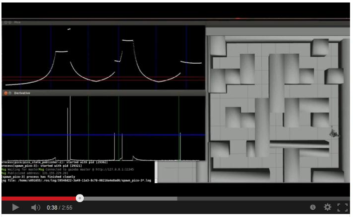
Before we transform the LRF data using the Hough function, we check at which type of surroundings we are dealing with. There are a number of possibilities, which are displayed in figure 8.

Using the laser range data, we can distinguish these situations by analyzing their values. Each situation has an unique amplitude-angle characteristic. We can generalize variations on the situations by assuming that a junction exit will reach a scanning range value above r_max. Setting the limit at r_max and thus truncating the scanning values will return characteristic images for each junction type:

Fig: Truncated LRF data (horizontal axis: scan angle, vertical axis: scan range)

If the average value (angle) of the truncated tops reach setpoint values (i.e. 0, 90, 180 degrees) w.r.t. the y axis we know what kind of junction we are dealing with. Now that we can identify the type of surroundings, we can tell if we have to navigate in a straight manner (corridor) or if we need to navigate towards an exit. With this information we can send messages to our motion node. So if we look at the figure above, we can identify three seperate exits.

The possible junction types are:

Fig 5:Different types of junctions

Fig

Fig

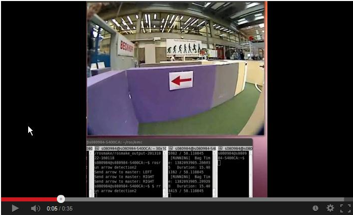
Arrow recognition

The pseudocode for the arrow recognition software is displayed in the following graph:

Fig:Pseudocode for arrow recognition

We first convert the video (bag) from red, green and blue (RGB) to black and white (BW). Next, we apply a blur filter and a Canny edge detector. We now have the countours displayed as displayed in step 2 of figure (XXX). Next, we apply a Hough transform to this countour. The options are tweaked such that only the arrows tail and head is found by the Hough transform. Now we have arrived at step 3 of figure (XXX). Next, we calculate the gadient ([math]\displaystyle{ \frac{dy}{dx} }[/math]) and average x-value (indicated by the points). We couple these values and then we sort these by the magnitude of the the of each linecouple this to the corresponding average x value of each li

Fig:Steps involving arrow recognition

Fig:arrow properties

Each of these have multiple variants as each exit can be a dead end.

Results

Now PICO is equiped with arrow recognition, junction detection, dead end detection (skips dead end corridors) and a wall follower. This is displayed in the video below.

References

• A. Alempijevic. High-speed feature extraction in sensor coordinates for laser rangefinders. In Proceedings of the 2004 Australasian Conference on Robotics and Automation, 2004.
• J. Diaz, A. Stoytchev, and R. Arkin. Exploring unknown structured environments. In Proc. of the Fourteenth International Florida Artificial Intelligence Research Society Conference (FLAIRS-2001), Florida, 2001.
• B. Giesler, R. Graf, R. Dillmann and C. F. R. Weiman (1998). Fast mapping using the log-Hough transformation. Intelligent Robots and Systems, 1998.
• Laser Based Corridor Detection for Reactive Navigation, Johan Larsson, Mathias Broxvall, Alessandro Saffiotti http://aass.oru.se/~mbl/publications/ir08.pdf