Embedded Motion Control 2013 Group 5

Group members

Name:	Student ID:
Arjen Hamers	0792836
Erwin Hoogers	0714950
Ties Janssen	0607344
Tim Verdonschot	0715838
Rob Zwitserlood	0654389

Tutor:
Sjoerd van den Dries

Planning

Weekly meetings

DAY	TIME	PLACE	WHAT
Monday	11:00	OGO 1	Tutor Meeting
Monday	12:00	OGO 1	Group meeting
Friday	11:00	GEM-Z 3A08	Testing

Deadlines

DATE	TIME	WHAT
September, 25th	10:45	Corridor competition
October, 23th	10:45	Final competition
October, 27th	23:59	Finish wiki
October, 27th	23:59	Finish peer review

Log

Week 1:

• Installed the software

Week 2:

• Did tutorials for ROS and the Jazz simulator
• Get familiar to 'safe_drive.cpp' and use this as base for our program
• Defined coordinate system for PICO (see Figure 1)

Week 3:

• Played with the Pico in the Jazz simulator by adding code to safe_drive.cpp
• Translated the laser data to a 2d plot
• Implemented OpenCV
• Used the Hough transform to detect lines in the laser data
• Tested the line detection method mentioned above in the simulation (see Figure 2)
• Started coding for driving straight through a corridor (drive straight node)
• Started coding for turning (turn node)

Week 4:

• Reorganize our software architecture after the corridor competition
• Created structure of communicating nodes (see Figure 3)
• Finish drive straight node (see Figure 4)
• Finish turn node
• Started creating a visualization node

Week 5:

• Finish visualization node
• Started creating node that can recognize all possible junctions in the maze (junction node)
• Started creating node that generates a strategy (strategy node) (see Figure 5)
• Tested drive-straight and turn node on Pico, worked great!

Week 6:

• Finished junction node (see Figure 6)
• Started fine tuning strategy node in simulation
• Tested visualization and junction node on Pico, worked fine!

Week 7:

• Finished strategy node (in simulation)
• Tested strategy node on Pico, did not work as planned
• Did further fine tuning of strategy node

Week 8:

• Simulation ok, tested ± 30 junctions
• All nodes communicating properly w.r.t. each other

Software architecture

The software architecture is shown in figure 3. In this section the architecture is explained in more detail. First we present an overview of all nodes, inputs and outputs. Then the most challenging problems that have to be tackled to solve the maze and the solutions are discussed.

Overview nodes

The software to solve the maze is build around the strategy node. This node receives all the information that is needed to solve the maze, and sends information to the nodes that actuate Pico. An overview of all nodes is given below. The column "PROBLEMS SOLVED" give a short description of the problems that are solved in the node.

NAME	INPUT	OUTPUT	PROBLEMS SOLVED
Strategy	*Laser data *Junction data *Turn data	*Command for left, right or straight	*Finding the next best step
Junction	*Laser data	*Type of junction	*Junction recognition
Turn	*Command for left, right or straight *Laser data	*Velocity command	*Localization *Control turning motion
Drive straight	*Command for left, right or straight *Laser data	*Velocity command	*Localization *Control straight drive motion
Arrow detection	*Odometry data	*Command for left or right	*Arrow recognition

The integration of the nodes can be visualized using rxgraph, which displays all used nodes and their mutual communication. This is done in figure 4.1a.

Fig 4.1a:Total software architecture

Design choices

During the entire development proces we made a number of design choices. Major decisions were made collectively. This was done by small brainstorm sessions and trial-and-error iterations. Smaller, more detailed design choices were made mostly indivudually when defining the code and are not discussed here.

At first we all agreed on a coordinate system for pico and decided that all control should be, if possible, based on feedback. Our opinion was that feedforward (driving/turning for several seconds) is not the way to go. The coordinate system is depicted in the figure below:

Figure 4.2a: PICO coordinate system

Prior to the corridor competition we dissected the work in two parts: driving straight and turning. Together these would be able to let PICO drive through the corridor. The group was split in two to work on these seperate parts. For the straight drive part we looked at the potential field algorithm and the hough tranform and decided to implement the Hough algorithm, since it is easier to implement and the hough transform also returns physical data in terms of dimensions of its surroundings (lines), which might come in use later. As for the second part, the turning algorithm, we used the derivative of the laserscan data to find peaks and thus identify corners. Once a exit was detected, we continued driving until the distance between the found corners was nearly equal.

After the corridor competition all code was still in a single file, and since we had to expand it with more algorithms we decided to re-organize the structure by creating seperate nodes and agreed on a strict input-output for each node. These nodes are displayed in table 4.1a, but at this time there was not yet a arrow/junction detection.

Now we started on a new turning and driving straight algorithm, because the first one did not work well enough. For the turning we have come op with a homebrew solutionn (XXX verwijzing naar) instead of turning for a given time (no feedback) or using odometry (false feedback). For the straight driving we use the hough from the openCV functions & libraries.

When these functions were completed we started to expand the software with extra nodes, Strategy, Junction and Arrow detection. To do this we first collectively discussed the approach for these nodes and determined the possible junctions PICO could encounter. As the deadline (maze competition) was coming closer we decided to first build a wall follower and then add extra options to this to make PICO smarter. So the plan was to first build a wall follower which can recognize dead ends and avoid these (which we call wall follower++), and if there was any spare time we could implement a mapping algorithm.

For the arrow detection we chose for a gradient based search algorithm. At first we had another one (based on outer positions of points on the arrow) but this was not usable when the arrow was tilted. The gradient based algorithm is more robust, so we used that one. We decided not to use the outcome of the arrow node in the strategy node since it may cause problems. This problem can best be recognized when visualized:

Figure 4.2b: infinite trajectory

When we would use a (semi) wall following algorithm but also implement the arrow detection in the strategy the result may be an infinite loop. This occurs when there are multiple paths that lead towards the exit. For example in the figure, if we prefer PICO to make right turns but take a single left (as suggested by the red arrow A), PICO will continue to go right after this left turn and as a result, be stuck on this "island" in the maze. For other directions an anologous situation can be depicted.

Strategy node

The goal of this competition is to solve the maze. The strategy node contains the plan of action to achieve this goal. The name of the strategy that is used is: Wall follower ++. This is basically a wall follower to the left but with the extension of dead end check. This will be explained in more detail later on. Figure 4.3a is a schematic representation of the strategy that is used. It is an ongoing loop which gets all the input data at the beginning of one cycle and ends the cycle with sending a command of what Pico should do. There is one exception in this ongoing loop, and that is when Pico is turning. More information about this exception is given later. Next the scheme in figure 4.3a is discussed.

Fig 4.3a: High level software architecture

It all starts with a position check, the node will determine whether Pico is in a corridor or at a junction. When Pico is in a corridor it will send a command to drive straight trough the corridor. The straight-drive node react on this command a will control the motion of Pico. When Pico is at a junction, the strategy node will first check what type of junction it is. This information is given by the junction node. When the junction type is clear, the strategy node will make a decision based on the scheme in figure 4.3b, this is a scheme of a standard wall follower. But as mentioned above it is extended with a dead end detector.

Figure 4.3b: Strategy, steps for driving

This means that when Pico has the possibility to go left, it will first be checked whether the corridor on the left is a dead end or not. When it is, the option to go left will not be take into account. So when Pico is at a junction it actually checks if there is a new junction after the current junction. Basically the strategy node is able to look two junctions ahead and makes a decision based on that information. When the decision is made, the strategy node will send a command to the turn node which controls the turn motion. This is the point when the ongoing loop holds for a while. The turn node will make shore that Pico turns the way the strategy node has commanded and will give a command back when the turn is completed. After that command the strategy node will continue the loop. So what the strategy node does is collect all input signals, decides what would be the best step to take to solve the maze and commands either to the straight-drive or turn node to control the motion. The special feature of the Wall follower ++ strategy is that it makes a decision based on the information that is gathered by looking two junctions ahead.

Drive straight node

Pico is driving through a rather narrow corridor and may not hit the wall. So when Pico is between two walls (this is determined in our turn and strategy node) the drive straight node is activated until pico is on a junction again. This node lets pico drive parallel to the wall and in the middle of the corridor. This is done by the following algorithm/pseudo code.

1. Create black-white image from the laserdata.

• The laserpoints will be white the rest black.
• Pay attention to the orientation of the picture.

2. Find lines through opencv function HoughlinesP()

• These will correspond to the walls.
• Returns (x,y) coordinates of begin and endpoints of the lines.
• Coordinate system in top left corner, positive x axis to the right, positive y down.

3. Calculate angle of the lines 'theta' , and length 'd' of a vector perpendicular to the line. See figure (..)

• Express these in the 'pico' coordinate system.

4. Pick the closest wall

• Based on the smallest 'd'.

5. Find the opposite wall

• Using 'theta' of the closest wall, the index in the laserdata of the closest point is calculated.
• Since the walls should be about parralel the same theta is used to find the index of the opposite wall.

6. Find middle of the corridor 7. Calculate drive angle

• Using the distance to the middle and a arbitrary distance along the corridor we find 'phi'.
• Our drive angle will be 'theta', to get parallel to the wall, plus 'phi' to turn towards the setpoint in the middle of the corridor.

8. Send the drive angle.

• the drive angle is set to a node called actuate. This node sets an x speed and uses the drive angle as the z-rotation speed.

As discussed above, the setpoint generator can be visualized as following:

Figure 4.4a: Setpoint generation

Turn node

Inputs:

• Laserscan
• Odometry
• Decision
• Junction

Outputs:

• Velocity
• rt-Image
• Booleans:
  • Request decision from strategy node
  • Request decision from arrow detection node
  • Turned 90 degrees

Fig 4.5a: Possible junctions

Junction node

Our strategy is mainly based on the decisions pico can make at each junction. Therefore a Junction node is realised, which is able to detect all 8 different types of junctions, see figure 4.6a. Also he can detect a dead end of corridor. Detecting dead ends in the beginning of a crossing is very usefull for solving the maze fast. No time is lost for driving into these blind corridors. The junction node only listens to the laser data and a request send by the strategy node.

Fig 5:Different types of junctions

Fig 4.6a: Different types of junctions

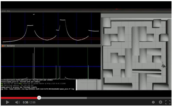
First of all, the junctions are detected. The regions for detecting left, straight and right corridors are determined and can be seen in Fig. 4.6b as blue vertical lines. The three humps in the graph are the three ways in the crossing of figure 4.6d. All junctions have a unique distance-angle characteristic. Therefore three booleans are used for determining humps right, straight or left. If a significant percentage laser points in one region is higher than the red threshold line, the hump is detected as a corridor and the corresponding boolean is set high. The three booleans are converted to an integer value and is published on demand of the strategy node.

Fig 4.6b: Laser Data, distance-angle characteristic

To detect dead ends, the derivative of the laser data is calculated and can be seen in figure 4.6c. This image is published and will be visualized in the visualization node. The peaks in the derivative are gaps in the laser data. Therefore large gaps represents a gap in the corridor . Also three regions and a threshold line can be obtained in the figure. This function also uses three booleans (Go_left Go_straight and Go_right). If a peak in a region is above the threshold, there is a possible way out and the bool is made true. The three booleans are also converted to an integer, which represents the possibilities of the junction. This decision integer is converted in the same way as the junction integer.

Fig 4.6c: Derivative of laser data

How the booleans are converted to the integers can be seen in table 4.6.1. The junction integer represents the type of junction, while the possibility contains the possibilties pico has at a crossing. The possibility value is a combination of the junction and the decision. For example, a junction of type 5 (left and right a corridor) can have blind ways left, right or both. Therefore it is possible that the junction message contains a 5 and the possibility message a 3. This possibility integer will be published on demand to the strategy node.

Left .	Straight .	Right .	Junction .	Possibility
1	0	0	1	1, 8
0	1	0	2	2
0	0	1	3	3, 8
1	1	0	4	1, 2, 4, 8
1	0	1	5	1, 3, 5, 8
0	1	1	6	2, 3, 6, 8
1	1	1	7	1 up to 8
0	0	0	8	8

table 4.6.1: Derivative of laser data

In total, there are 26 different combinations that can occur. At a 4 way crossing, junction is 7, there are 8 possible combinations! All these combinations are tested in simulation and the pico could detect all posiblilties very well as you can see in figure 4.6d, 4.6c & 4.6b. PICO sees three corridors and publishes a junction with value 7. But he can only go into the left or straigth corridor and therefore he publishes a possiblity with value 4.

Fig 4.6d: Example crossing (junction = 7, Possibility = 4)

Visualization node

As soon as we started programming an efficient way for debugging was chosen. Putting print statements everywhere is not very efficient, so we decided to visualize as much as possible. The standard library of C++ does not support visualization, so an extra library (OpenCV) was added already in the third week. This library contains visualization functions, but there are also many image processing functions that can be used in the arrow detection node and other functions. At the corridor competition we already had some visualization, but this was not implemented in a separate node. This was also the problem whereby we failed at the corridor competition. Due to the imshow() function, we were publishing the velocity message on a very low frequency, ± 5Hz instead of the desired 20 Hz. At that point we decided to make an independent visualization node which will be run on a separate laptop. Through this simple modification, the nodes which run on pico will publish and read at 20 Hz. The visualization node will read the topics at a lower 10Hz rate. The visualization node listens to three topics, which contains three images we show:

• The first image contains the xy graph pico sees, which is shown in figure 4.7a. This image shows the laser data converted to Cartesian coordinates and is used by the drive-straight nodes. The Hough-transformation uses this image for detect the nearest lines.
• The laser data will be plot in the second image, which is shown in figure 4.6b. The distance is plotted against the angle on the y and x axis respectively. This plot will be used to define thresholds and regions for turning and junction detection.
• The last image contains the derivative of the laser data, which is shown in figure 4.6c. The absolute value of the derivative function is used to detect gaps in a corridor. These gaps are used by the junction decision making function.

Fig 4.7a: Cartesian reconstruction of laserdata

By visualizing as much as possible, debugging went quit fast. Fine-tuning the interesting regions and the thresholds went much easier. The threshold values for example must be lower in the real maze and higher in the simulation. More insight in the data is obtained when the data is plotted, because some strange behavior like noise in the laser data was seen directly. Also the images are used in the presentation and on the wiki page, for clarification. A picture is worth as much as thousand words.

Arrow recognition node

As mentioned before, we did incorporate arrow recognition in the software. We kept the results on a scrict information-output basis (using a cout//). The arrow recognition software was constructed as a seperate node which communicates with the central strategy node. The architecture of this node is displayed in the figure below in chronological order:

fig 4.8a):Pseudocode for arrow recognition

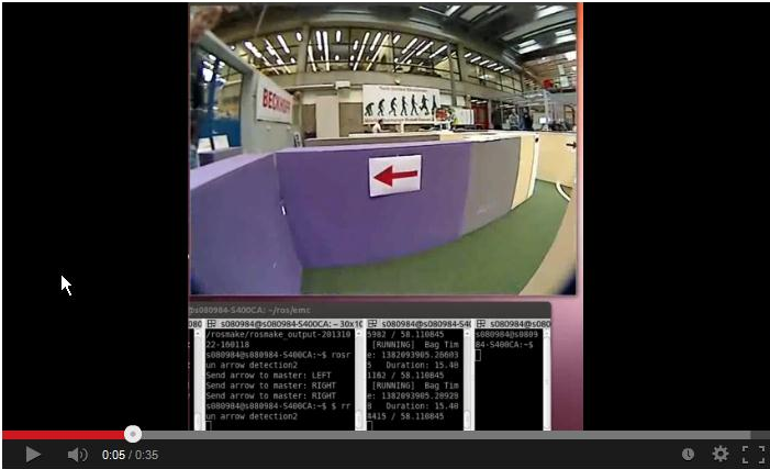
When online, these functions output their data to the GUI as displayed in figure 4.8b.

fig 4.8b):Steps involving arrow recognition

We first convert the video (bag, see step 1 of figure 4.8b) from red, green and blue (RGB) to black and white (BW). Next, we apply a blur filter to the image. This is a openCV function and smoothes the image. After this a Canny edge detector is applied. We now have the countours displayed as displayed in step 2 of figure 4.8b. Next, we apply a Hough transform to this countour. The options are tweaked such that only the arrows tail and head is found by the Hough transform. Now we have arrived at step 3 of figure 4.8b. Next, we calculate the gadient ([math]\displaystyle{ K_i=\frac{dy_i}{dx_i} }[/math], i=1..n, n=no. found lines) and average x-value (indicated by the points in figure 4.8c. We couple these values and then we sort these by the magnitude of the gradients. These variables are shown in the figure below.

Fig 4.8c):arrow properties

We want to compare the head of the arrow with its tail. If the average x position of the head is smaller than its tail we know it points to the left and vice versa to the right. We know that [math]\displaystyle{ K_1 }[/math] has the largest gradient and [math]\displaystyle{ K_n }[/math] the lowest. The tail is somewhere in between. So if we compare the average x corresponding to the maximum gradient with that of the median gradient we can find the orientation of the arrow by checking at which side (x) the maximum gradient is w.r.t. the median gradient.

Evaluation

Now PICO is equiped with arrow recognition, junction detection, dead end detection (skips dead end corridors) and a wall follower. This is displayed in the video below.

TEMPORARY CHAPTER: NOTES

NOTES MAY BE PUT HERE SO THESE CAN BE ADRESSED LATER (AFTER FINAL MEETING)

- unknown references are currently marked with XXX

- planning section might be irrelevant??

References

• A. Alempijevic. High-speed feature extraction in sensor coordinates for laser rangefinders. In Proceedings of the 2004 Australasian Conference on Robotics and Automation, 2004.
• J. Diaz, A. Stoytchev, and R. Arkin. Exploring unknown structured environments. In Proc. of the Fourteenth International Florida Artificial Intelligence Research Society Conference (FLAIRS-2001), Florida, 2001.
• B. Giesler, R. Graf, R. Dillmann and C. F. R. Weiman (1998). Fast mapping using the log-Hough transformation. Intelligent Robots and Systems, 1998.
• Laser Based Corridor Detection for Reactive Navigation, Johan Larsson, Mathias Broxvall, Alessandro Saffiotti http://aass.oru.se/~mbl/publications/ir08.pdf