Mobile Robot Control 2024 Robocop: Difference between revisions
(→Group members: Arif: Exercise 1 results using one method.) |
|||
| (10 intermediate revisions by 3 users not shown) | |||
| Line 24: | Line 24: | ||
|1859234 | |1859234 | ||
|} | |} | ||
=Exercise 1= | |||
== Exercise 1 == | |||
=== Method 1 - Arif === | === Method 1 - Arif === | ||
| Line 31: | Line 32: | ||
Some experimentation was done to test different speeds and thresholds for the stopping range values. When the speed was higher than the stopping range value the robot would actually crash into the wall first before stopping, and if it was lower then the robot would stop slightly farther away from the wall. However, this only seemed to be the case when the stopping value was very low (e.g. 0.1), but increasing it to 0.2, for example, allowed the speed to be increased to 0.4 without any crashing. | Some experimentation was done to test different speeds and thresholds for the stopping range values. When the speed was higher than the stopping range value the robot would actually crash into the wall first before stopping, and if it was lower then the robot would stop slightly farther away from the wall. However, this only seemed to be the case when the stopping value was very low (e.g. 0.1), but increasing it to 0.2, for example, allowed the speed to be increased to 0.4 without any crashing. | ||
== Exercise 2 == | |||
===Method 1 - Arif=== | |||
[[File:Dont crash ex2 map1.png|thumb|268x268px|Method 1 on Map 1.]] [[File:Dont crash ex2 map2.png|thumb|273x273px|Method 1 on Map 2.]] | |||
The previously described method was tested on the two provided maps with input speeds of (0.3, 0, +-0.3) and a stopping value of 0.2. With both maps the robot successfully came to a stop before crashing, although it struggled when driving into a corner and stopped much closer to the wall than it did in previous tests. | |||
== Practical Exercises 1 == | |||
== Local Navigation == | |||
=== Dynamic Window Approach === | |||
===== The approach ===== | |||
The approach can be divided in the following sequential steps: | |||
# '''Calculate the union between the Possible (angular) Velocities (Vs, Ws) and the Reachable (angular) Velocities (Vd, Wd)''' | |||
#* EXPLAIN HOW | |||
# '''Iterate through the discretized values (''v, w'') of the union of Vs, Vd and Ws and Wd:''' | |||
## '''Calculate the Admissable (angular) Velocities (Va,Wa) using ''v'' and ''w''''' | |||
##* EXPLAIN HOW | |||
## '''Check if ''v'' and ''w'' are also in Va and Wa, if this is the case:''' | |||
##* '''Calculate the optimization function value. If this value is higher than the previous optimization value, set the current ''v and w'' to ''v_final'' and ''w_final''''' | |||
##** EXPLAIN HOW | |||
# '''Return ''v_final, w''_final''' | |||
Our approach for the Dynamic Window Approach (DWA) is that we first make a list of samples that fit inside the possible velocity limit (Vs) and reachable velocity and acceleration constraints (Vd). After which we | |||
===== Questions ===== | |||
'''1. What are the advantages and disadvantages of your solutions?''' | |||
Advantages: | |||
# By constantly calculating possible trajectories it is able to avoid dynamic and static obstacles. | |||
# By including the robot acceleration and deceleration constraints it ensures for a smooth navigation without abrupt movements. | |||
Disadvantages: | |||
# DWA may get trapped in a local minima. | |||
# There is a high computational load in calculating the multiple trajectories in real-time | |||
'''2. What are possible scenarios which can result in failures?''' | |||
# Like mentioned in question 1 DWA can get trapped in a local minima. | |||
#* '''Solution:''' Include the global planner so it doesn't drive into a local minima | |||
# We also encounter some problems when the robot is driving to a straight wall and can't decide with direction to take. (see video: https://gitlab.tue.nl/mobile-robot-control/mrc-2024/robocop/-/blob/main/videos_and_photos/dwa_straight_wall.mp4) | |||
#* '''Solution:''' Increase Ks and decrease Kh so the robot is less constrained to drive directly towards the goal. | |||
'''3. How are the local and global planner linked together?''' | |||
Latest revision as of 12:14, 24 May 2024
Group members:
| Name | student ID |
|---|---|
| Matijs van Kempen | 2060256 |
| Luc Manders | 1729225 |
| Marc Quelle | 2044749 |
| Marijn Ruiter | 1489496 |
| Luke Alkemade | 1581643 |
| Arif Ashworth | 1544632 |
| Abhidnya Kadu | 1859234 |
Exercise 1
Method 1 - Arif
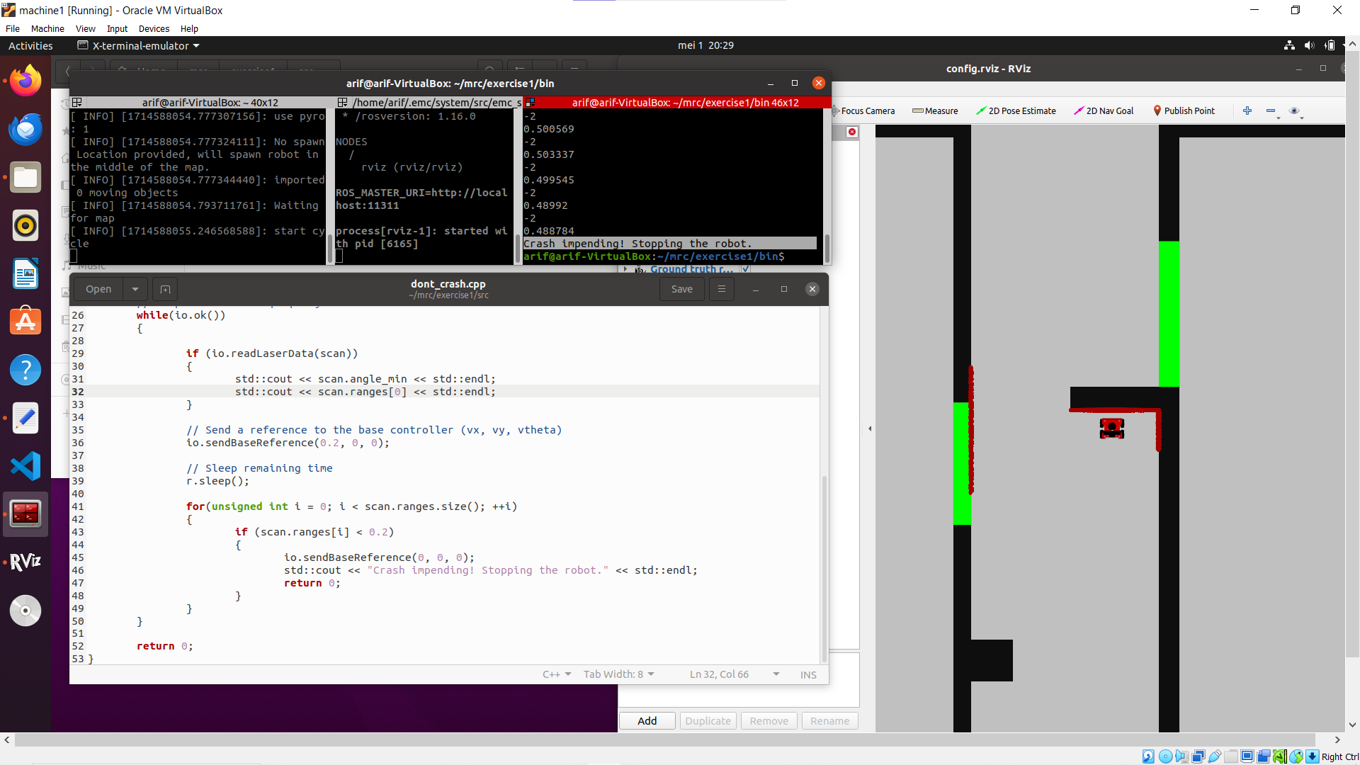
In this method the LaserData struct is used to track the measured distances from the walls to the robot. To make the robot drive forward the sendBaseReference command is used, and the robot moves in the x direction at a speed of 0.2. Once it reaches the wall in front of it and the range values drop to below 0.2, motion is halted and a message is printed to the screen before exiting the program.
Some experimentation was done to test different speeds and thresholds for the stopping range values. When the speed was higher than the stopping range value the robot would actually crash into the wall first before stopping, and if it was lower then the robot would stop slightly farther away from the wall. However, this only seemed to be the case when the stopping value was very low (e.g. 0.1), but increasing it to 0.2, for example, allowed the speed to be increased to 0.4 without any crashing.
Exercise 2
Method 1 - Arif
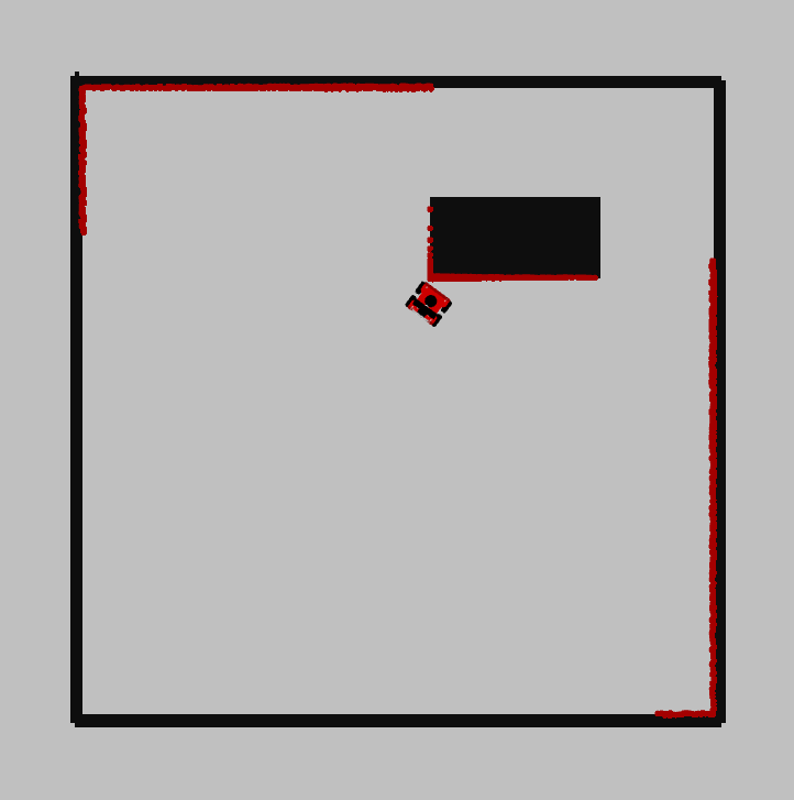
The previously described method was tested on the two provided maps with input speeds of (0.3, 0, +-0.3) and a stopping value of 0.2. With both maps the robot successfully came to a stop before crashing, although it struggled when driving into a corner and stopped much closer to the wall than it did in previous tests.
Practical Exercises 1
Dynamic Window Approach
The approach
The approach can be divided in the following sequential steps:
- Calculate the union between the Possible (angular) Velocities (Vs, Ws) and the Reachable (angular) Velocities (Vd, Wd)
- EXPLAIN HOW
- Iterate through the discretized values (v, w) of the union of Vs, Vd and Ws and Wd:
- Calculate the Admissable (angular) Velocities (Va,Wa) using v and w
- EXPLAIN HOW
- Check if v and w are also in Va and Wa, if this is the case:
- Calculate the optimization function value. If this value is higher than the previous optimization value, set the current v and w to v_final and w_final
- EXPLAIN HOW
- Calculate the optimization function value. If this value is higher than the previous optimization value, set the current v and w to v_final and w_final
- Calculate the Admissable (angular) Velocities (Va,Wa) using v and w
- Return v_final, w_final
Our approach for the Dynamic Window Approach (DWA) is that we first make a list of samples that fit inside the possible velocity limit (Vs) and reachable velocity and acceleration constraints (Vd). After which we
Questions
1. What are the advantages and disadvantages of your solutions?
Advantages:
- By constantly calculating possible trajectories it is able to avoid dynamic and static obstacles.
- By including the robot acceleration and deceleration constraints it ensures for a smooth navigation without abrupt movements.
Disadvantages:
- DWA may get trapped in a local minima.
- There is a high computational load in calculating the multiple trajectories in real-time
2. What are possible scenarios which can result in failures?
- Like mentioned in question 1 DWA can get trapped in a local minima.
- Solution: Include the global planner so it doesn't drive into a local minima
- We also encounter some problems when the robot is driving to a straight wall and can't decide with direction to take. (see video: https://gitlab.tue.nl/mobile-robot-control/mrc-2024/robocop/-/blob/main/videos_and_photos/dwa_straight_wall.mp4)
- Solution: Increase Ks and decrease Kh so the robot is less constrained to drive directly towards the goal.
3. How are the local and global planner linked together?


