Mobile Robot Control 2020 Group 4

Group Members

Name	Student Number	Email
M. Katzmann	1396846	m.katzmann@student.tue.nl
B. Kool	1387391	b.kool2@student.tue.nl
R.O.B. Stiemsma	0852884	r.o.b.stiemsma@student.tue.nl
A.S.H. Vinjarapu	1502859	a.s.h.vinjarapu@student.tue.nl
D. van Boven	0780958	d.v.boven@student.tue.nl
R. Konings	1394819	r.konings@student.tue.nl

Introduction

Welcome to the wiki page of group 4 of the 2020 Course Mobile Robot Control. The goal of this course is to design and implement software to the PICO robot which allows it to complete two different challenges, the escape room challenge and the hospital challenge. Both challenges are in a simulated environment and should be succesfully completed by the PICO robot autonomously. A design document is delivered before participating in these challenges which describes the overal architecture of the software.

Figure 1: Example maps of the escape room challenge (left) and hospital challenge (right)

Design document

The design document describes the architecture of the software. The document is divided into the requirements, functions, components, interfaces and specifications and is relevant for both the escape room challenge and hospital challenge. However, the document should be considered a guidance for both challenges, and the initially declared functions and software architecture are subject to change as the project progresses.

Escape room challenge

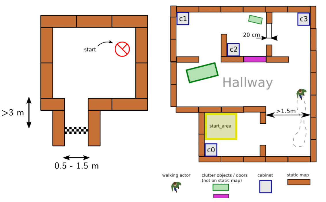
This challenge is designed as an itermediate challenge. The goal of the escape room challenge is to have PICO escape a rectangular room by exiting this said room through a corridoras fast as possible. The dimensions of this room are unknown as well as the initial position and rotation of the PICO robot. The corners of the room are not perpendicular but vary around 90 degrees. A simple example map of the room iss provided before the challenge, which can be seen in figure 1. During the escape of the PICO robot, walls, static and dynamical objects may not be touched, but slightly touching is allowed.

Hospital challenge

The goal of the hospital challenge is to have PICO autonomously manoeuvre through a simulated hospital environment. The hospital environment consists of multiple rooms and a hallway. Each room contains cabinets and the objective is for PICO to deliver medicine from one cabine to another, where the order will be defined by the judges. Similar to the escape room challenge, the dimensions of the map and the initial position and rotation of the PICO are unknown. However, the starting room will be provided beforehand. During the delivering of medicine by PICO, a handful of static and dynamical objects will be in PICO's way. It is PICO's job to avoid collision with any objects or walls and deliver the medicine in the correct order as fast as possible. An example map of the hospital environment is provided, which can be seen in figure 1.

Design Document

This document describes the design of a PICO application. There are two competitions for the robot to complete. The escape room competition, where the robot needs to escape out of a rectangular room, without bumping into a wall. And the robot needs to complete the hospital competition, where the robot needs to maneuver through a hospital, where it has to avoid obstacles. This document should be considered a guidance for both challenges, and the initially declared functions and software architecture are subject to change as the project progresses.

Requirements

Figure 2: Requirements tree escape room (dotted area) and hospital room

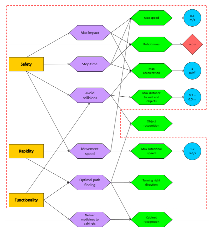
A requirement tree is constructed with the requirements from the stakeholders of the project. The stakeholders are the customer, the hospital employees and the developers of the robot. From here on, the environmental requirements, indicated with the orange boxes, have been acquired. From these environmental requirements, the border requirements, indicated with the purple boxes, have been acquired. Lastly, the system requirements have been acquired, indicated with the green boxes. Some of the green boxes have a set value assigned, indicated with a blue ball. And other system requirements are out of scope for the project team, indicated with a red square. The requirement tree of the hospital challenge can be seen in figure 2. The requirement tree of the escape room is indicated with the red dotted line.

The values assigned to system requirements are still subject to change as the project progresses. In addition, two values have not been chosen yet. Namely the maximum acceleration and the maximum distance to walls and objects. The maximum acceleration will be chosen accordingly once more information of the robot is available. The maximum distance to walls and objects has been chosen between a range from 0.1 and 0.5 meter and will also be chosen accordingly later on when more information is available.

Functions

In this section, the proposed architecture is described by means of its constituent functions and their relationships (interfaces) between one another.

PICO interfaces

These are all low-level interactions consisting mostly of calls to the IO API (which represents communication with PICO).

• Actuate(v, u, th): Casts a desired velocity profile [x′, y,theta″] to the robot.
• getLRF(): Pulls LRF data from the robot. Returns a laserdata struct.
• getODO(): Pulls odometry data from the robot. Returns an OdometryData struct.

Mapping

This section describes the outlines of the internal map model and its learning process.

• seeLocal(Laserdata): Interprets laserdata as a local vision envelope, and stores the outcome locally.
• loc2glob(): Transforms local sensor data into a global perspective using calibration elements (e.g. intersections of wall lines).
• tf2map(): Transforms sensor data (in a global coordinate system) to Mapdata, which involves rasterizing the received data.
• integrate(): Compares and contrasts new data with old data, and modifies (and/or expands) the global map model accordingly.

Navigation

This section covers the system functionalities responsible for (intelligent) navigation. All functions here have read access to the world model’s internal map and LRF envelope.

• localize(): Deducts the PICO’s current location in the map model based on its most recent LRF data.
• pathfind(x, y): Employs a pathfinding algorithm to find a combination of rotations and straight motions (longitudinal or sideways) that will bring the PICO from its current location to the global coordinate (x, y). Returns a PathData struct which describes the intended locations, and necessary rotations and local (x, y) motions to reach them.
• nextTrajectory(): Takes the next first data from PathData, and calculates the necessary velocity profiles and timings to achieve the desired motion smoothly. Returns this as a Trajectory struct.
• compensate(): Checks the PICO’s current location compared to its intended location within the planned path, and determines whether compensation is needed in the sense of adjusting the path, the PICO’s position, or recomputing the path.

Supervisor

This section covers the governing control logic of the proposed system. The idea is that the supervisor makes choices, tunes parameters, and controls flow-of-command within remaining code depending on its mode, and changes modes dynamically. Modes are described here as functions, but may end up in a different form during implementation.

• init(): Initializes the robot, checks (as far as possible) whether safe operation is possible. Sets the mode to scout.
• scout(): PICO is uncertain about its surroundings, and hence scans its surroundings, moving as little as possible in doing so. In this mode, safety parameters are conservative. Once a useful feature (such as a door) is found, or map confidence improves enough for PICO to feel safe, control is yielded to the move mode. If all exploration options are exhausted and PICO is still uncertain, control is instead yielded to wait.
• move(): PICO knows enough, and knows where it wants to go. This mode sets safety margins much more aggressively than scout mode, and looks to move long, efficient motions in pursuit of PICO’s intended destination. During motion, PICO keeps updating its map, and reverts to scout mode if certainty dips to unacceptable levels.
• wait(): PICO decides its goal is currently impossible. Waits, and occasionally returns to scout mode to see if the situation has changed.
• act(): An empty token mode to represent PICO arriving at a destination and doing something there.

Interfaces

Figure 3: State Machine Representation

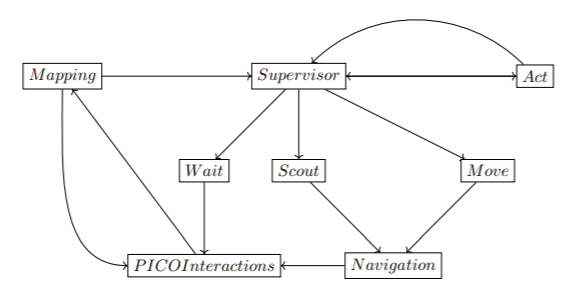
Keeping the aforementioned functionalities in mind, and given that the modes of the Supervisor module are represented here as separate locations for clarity’s sake, a rough depiction of the proposed system structure is shown in Figure 3.

Components

The hardware of the PICO robot used to smoothly execute the functions mentioned above, consists of the following components:

• Sensors
  • Laser Range Finder
  • Wheel encoders
• Actuators
  • Holonomic wheels
• Computer
  • IntelCore i7 Processor 8+ GB of DDR3 RAM

Specifications

System: PICO

• Maximum translational velocity: 0.5 m/s
• Maximum rotational velocity: 1.2 rad/s
• Wheel encoders used for odometry
• Laser Range Finder used for distance measurement
  • Measurable angle: 4 radians
  • Resolution: 0.004 radians

Environment

• Escape room challenge
  • Shape of the room is rectangular
  • PICO starts at a random position
  • Width of the corridor is between 0.5m to 1.5m
  • Finish line is more than 3m into the corridor whose orientation is perpendicular to the wall
  • Walls are not necessarily perfectly straight
  • Corners are not necessarily perfectly perpendicular
  • Challenge is to be finished within 5 mins

• Hospital challenge
  • Hallway is approximately 1.5m wide and is not necessarily straight
  • Doors in the hospital are 0.5m to 1m wide.(closed or open)
  • A random number of static and dynamic obstacles will be present throughout the hospital
  • Challenge is to be finished in 5 mins

Escape Room Challenge

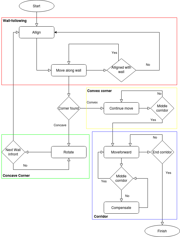
To safely get the PICO robot to the exit of the escape room, the strategy to implement a wall-follow algorithm is chosen. If the Algorithm is implemented successfully, it should be a safe and quick solution to the problem. The PICO will move to a wall, after which he will align perpendicular to the wall. When aligned to the wall, PICO will move left until it reaches either a wall or a gap. It will choose to rotate or drive into the gap accordingly. This algorithm was chosen because it is a reliable algorithm that, if implemented successfully, is safe and a relative quick escape.

The wall-follow algorithm is divided into the following sub-parts:

Figure 4: Flowchart escape room challenge

Step 1: The PICO moves forward

The PICO moves forward until it reaches a wall. The PICO will start at a random location inside the escape room. This means the robot can be anywhere inside the room. Thus, the first thing PICO does is move forward until it detects a wall getting closer. As the wall gets closer, the velocity of PICO decreases until it reaches a certain threshold from the wall, which means the PICO will stop moving.

Implementation

For this step, a simple function called goToWall(alignDistance) is constructed. This function lets PICO move forward while continuously checking if the minimum distance from PICO to any surrounding wall is smaller or equal to the given alignDistance. If this is the case, movement for the PICO stops and step 2 will be initiated.

Step 2: The PICO aligns to the wall

When PICO reaches the wall and completely stops moving, PICO starts rotating. It will rotate until it is perpendicular to the wall. This is achieved by having PICO stop rotating once the the middle LFR sensor has the smallest value. Here, the rotational velocity also decreases when the distance to the end point decreases.

Implementation

To align PICO to the wall as accurate as possible, the function alignWall(vx, vy, distWall) is constructed. Here, the rotation difference between the wall and the PICO is used to adjust the rotation speed of the PICO. The closer PICO is to the end goal, thus the rotational difference is getting smaller, the smaller the rotation speed is until it reaches the endgoal of being aligned perpendicular to the wall. After reaching perpendicularity, PICO continues with step 3.

Step 3: The PICO follows the wall

Once the PICO is perpendicular to the wall, it is ready to start following the wall. This is done by moving the PICO to the left until it detects a corner. If the PICO detects a convex corner, this means there is a corner approaching, and if the PICO detects a concave corner, this means there is a corridor approaching. The PICO will align to the new wall and repeat step 3 when there is a corner detected and it moves to step 4 if a corridor is detected.

Implementation

The function followWallTillNextWall() is constructed in such a way that PICO will go left after it is aligned to a wall. The function continuously checks if there is either a convex or concave wall approaching from the left. In case PICO detects a convex wall, it will use the function rotateTillNextWall(angle) until it is perpendicular to the new left wall and repeat step 3. In case of a concave PICO continues to step 4.

Step 4: The PICO detects corridor

The PICO drives a little further until the PICO is aligned to the exit. Once it is aligned to the corridor and feels safe enough to move, the PICO will move forward until the exit is reached.

Implementation

The function checkAllignmentCorridor(elementDiff) is created to move PICO beyond the first corner of the corridor entrance. It will check if PICO is in the middle of the corridor entrance by using the function checkIfInCorridor(). Once the PICO is aligned and ready to move, it will exit the corridor using function alignWithinCorridor(vx). This function makes sure PICO is aligned with respect to the left and right wall of the corridor and adjusts the x, y and rotation speed accordingly.

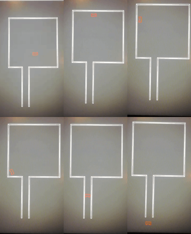
During the wall-follow algoritm, the PICO checks if it is too close to a wall and if it is well alligned at all times. The flowchart that is used for the escape room challenge is shown in figure 4.

Escape room trial run

Before going for the final challenge, the wall-follow algorithm has been tested using a trial map with corridor width set to the lower limit of 0.5m. As can be seen from the video below, the PICO has successfully made it through the narrowest corridor in the trial with this strategy.

Escape room challenge results

With the wall-following algorithm, the PICO achieved second place in the escape room challenge. The exit was reached within 27 seconds. The result of the challenge can be seen in the video. With the created algoritm, it can be seen that PICO firstly moves to the wall in front of him and stops when he is within the threshold range. Afther this, PICO perfectly aligns himself perpendicular to the wall, ready to move to the left. When moving to the left, first it encounters a convex wall, which means he rotates and aligns to the wall left of him. After the PICO is aligned to the new wall, it moves to the left until it encounters the corridor. Here, the PICO positions himself in front of the corridor. Once the PICO is positioned and feels it is safe enough to move, it drive through the corridor to the exit.

Hospital Challenge

[Under construction]

Software Architecture

The software design is explained in this section. An overview of the structure of the software is given and the different functionalities are listed. Such that the overall structure and connections in the software are clear. A detailed explanation and reasoning of the individual algorithms are given in the next section.

The software design is based on the different challenges that occur in the Hospital competition. This means that all the challenges, that at first sight can be deducted, are listed before a design is made.

To complete the hospital run the PICO should be able to plan a path between two given points. The path should be based on a map. The two given points, start and goal, are defined as a coordinate in this map. For this functionality, pathfinding, a costmap-based algorithm called A* is used.

The translation between the coordinates in the map and the real coordinates in the hospital should be constantly monitored. The relationship is not direct, because the odometry data has noise. This implies that this translation can not purely be based on odometry. On top of the odometry data, the LRF data can also be used to deduce the position of the robot. However, there is also some noise on the LRF data, so a combination of the odometry- and laser data should be used to deduce the position of the robot. A FastSLAM algorithm is used. This algorithm makes use of different landmarks in its surroundings. An algorithm to spot and link the local landmarks to the global landmarks is needed. A feature-detection algorithm is needed to accomplish this.

Based on the localization and the calculated path the pico should be able to move from its current position to a defined next position. During the movement, static and dynamic objects should be avoided at all times. A velocity-vector based algorithm can take this active avoidance into account via a so-called potential field.

The main algorithms of the software are A* algorithm for Pathfinding, FastSLAM for localization and orientation, velocity vector for path movement, a local potential field for obstacle avoidance, a feature detection, and a mapping procedure. These algorithms are the foundation of the whole software and the designs are based on these algorithms.

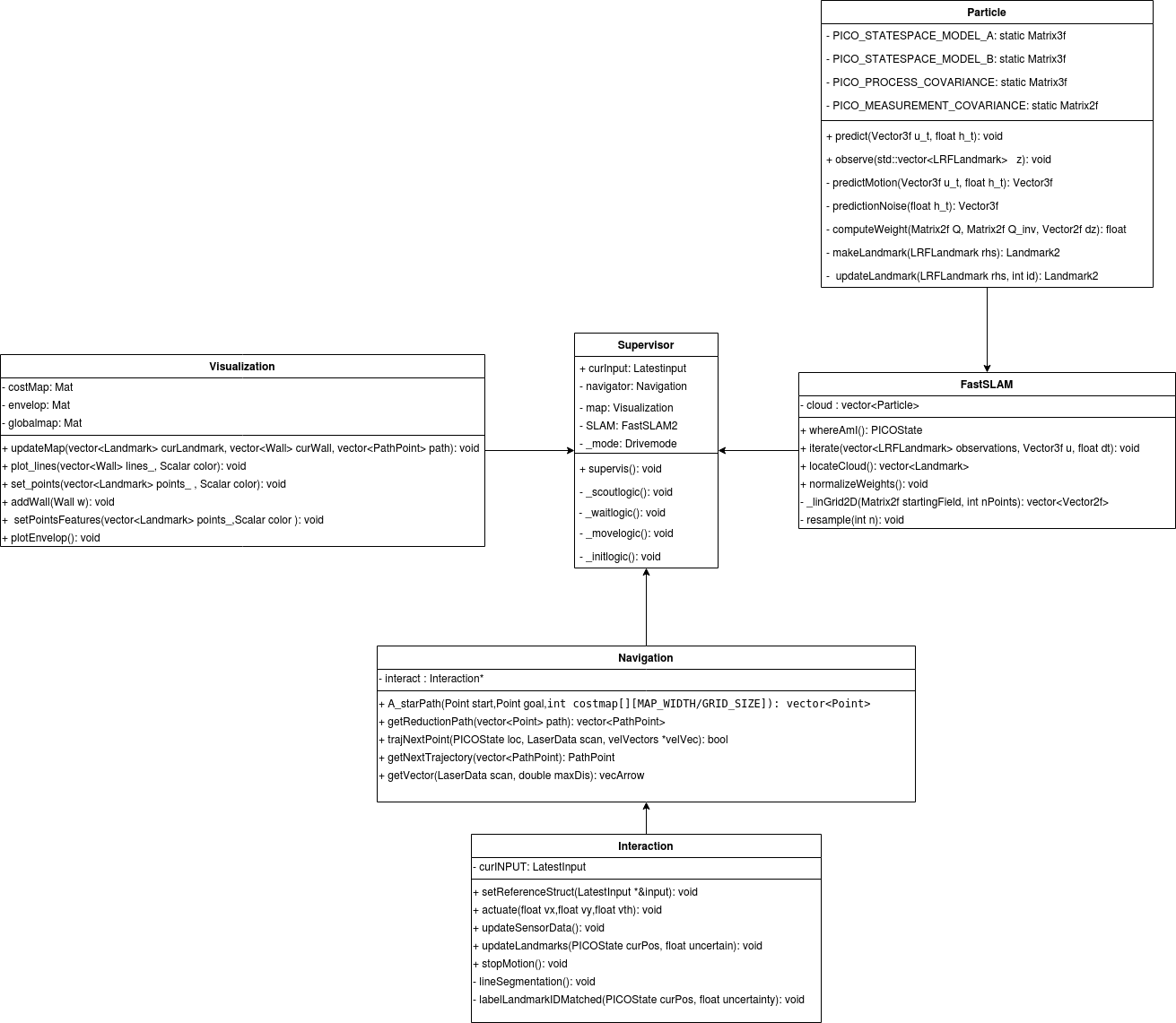
A class diagram is made to give an overview of the general structure of the software. The different above mentioned algorithms are grouped to form a class, with the intention to create a hierarchy. The supervisor class is created as the top class in the hierarchy structure. In this class, every other sub-classes are called. The supervisor class is divided into 5 modes, namely initialization, scout, move, wait, and act. Switching between these modes is done on the basis of the outcome of the function in the sub-classes.

The sub-classes that are directly underneath the supervisors are Navigation, FastSLAM, and Visualization. The abovementioned algorithms are divided into these sub-classes. The Navigation contains the A* global path planning, velocity vector based movement, a local potential field, and feature detection. The Navigation class has a sub-class named Interaction, which is the only connection point to the PICO robot. The reading of the sensors and the control of the movement takes place in this class. However, since these readings are needed in other classes a struct is made, which contains all the useful information based on the current readings. This struct is made in the supervisor class and is linked to the address of a similar struct in the Interaction class. The current readings and detected features are now available in the supervisor class and can be from there. The FastSLAM class is a class fully based on the FastSLAM algorithm with a sub-class Particle which plays an important part in the algorithm. The Visualization class is based on the visualization and maintaining the map of the environment.

Algorithms

For the Hospital Challenge, the design of the algorithm is divided into four parts: interaction, supervisory, mapping and navigation. Each part has its own functionality and needs to work with the other parts. This functionality is explained below:

Feature Detection

Feature Recognition

The goal of the feature recognition part of the software is to read PICO’s laser rangefinder data and interpret it in a way that is useful for the localization algorithm.

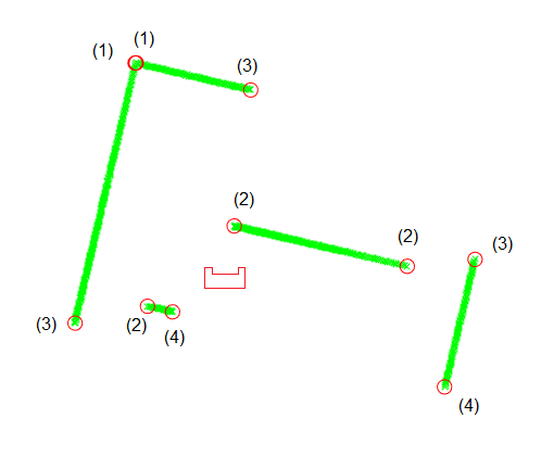
The first main function is to detect corners. The hospital consists of perpendicular straight walls. The localization algorithm uses the corners of these walls as landmarks. The rangefinder data is divided up in a number of straight line segments for the walls. The ends of these segments are, after a filtering step, seen as corner landmarks and saved.

The second main function is identifying the corners. The localization not only needs to know what corners PICO sees but also which corners those are. The supplied hospital map has a numbered list of the position of all corners. Using the PICO’s position the detected landmarks can be matched to the map landmarks and obtain their ID.

The feature recognition consists of the following algorithms:

1. Dividing the data points into segments
2. Designating the ends of segments as detected landmarks
3. Filtering the detected landmarks to reduce matching workload
4. Matching the detected landmarks to the map's landmarks

Segmentation

Figure [segmentation_figure]: The segmentation algorithm

The detected laser rangefinder data consist of an array containing 1000 radii, the corresponding angles of these points as seen from PICO are fixed quantities. Together they make up a local polar coordinate system. The segmentation algorithm uses these points in cartesian coordinates so a conversion step is used.

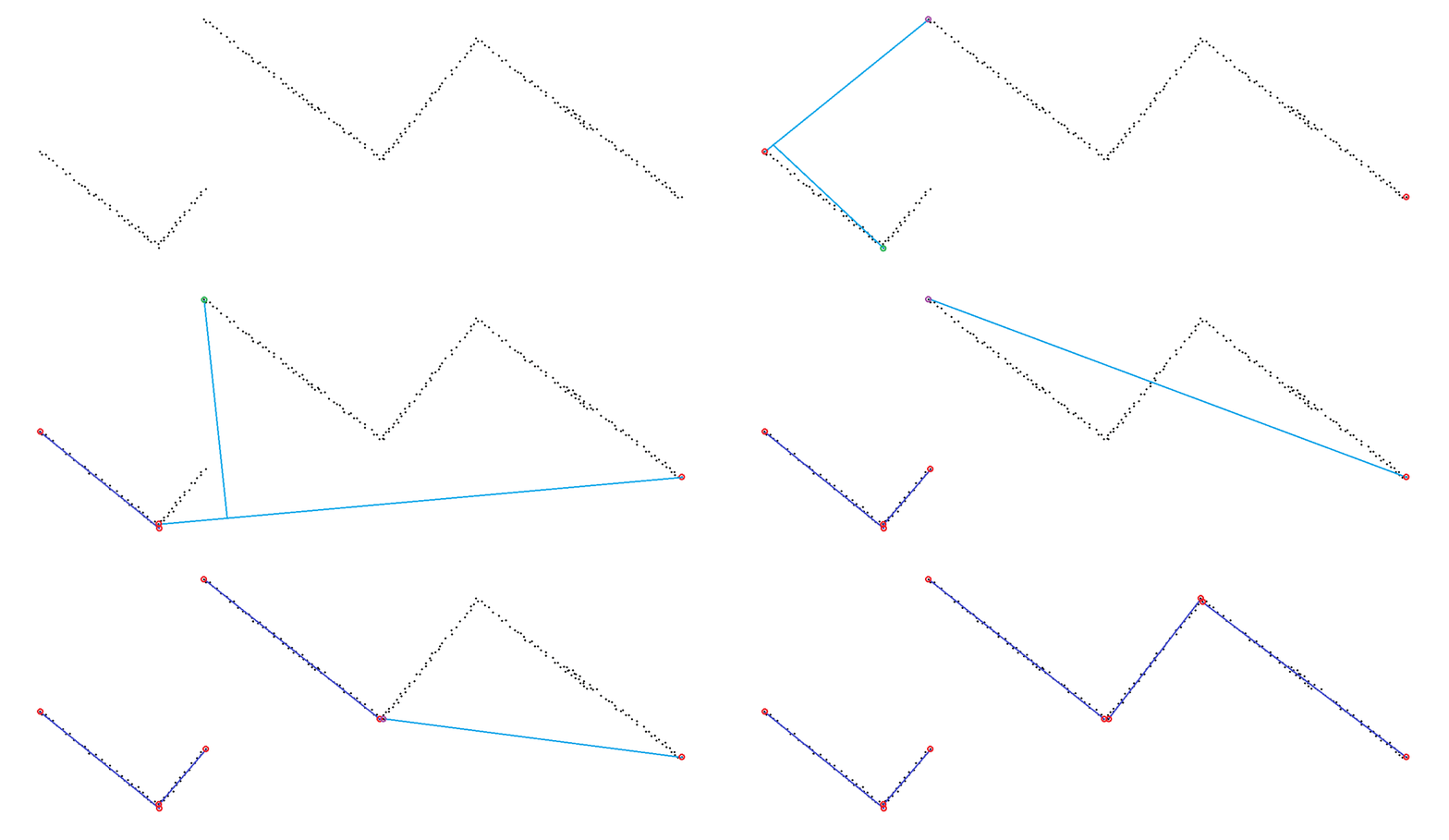
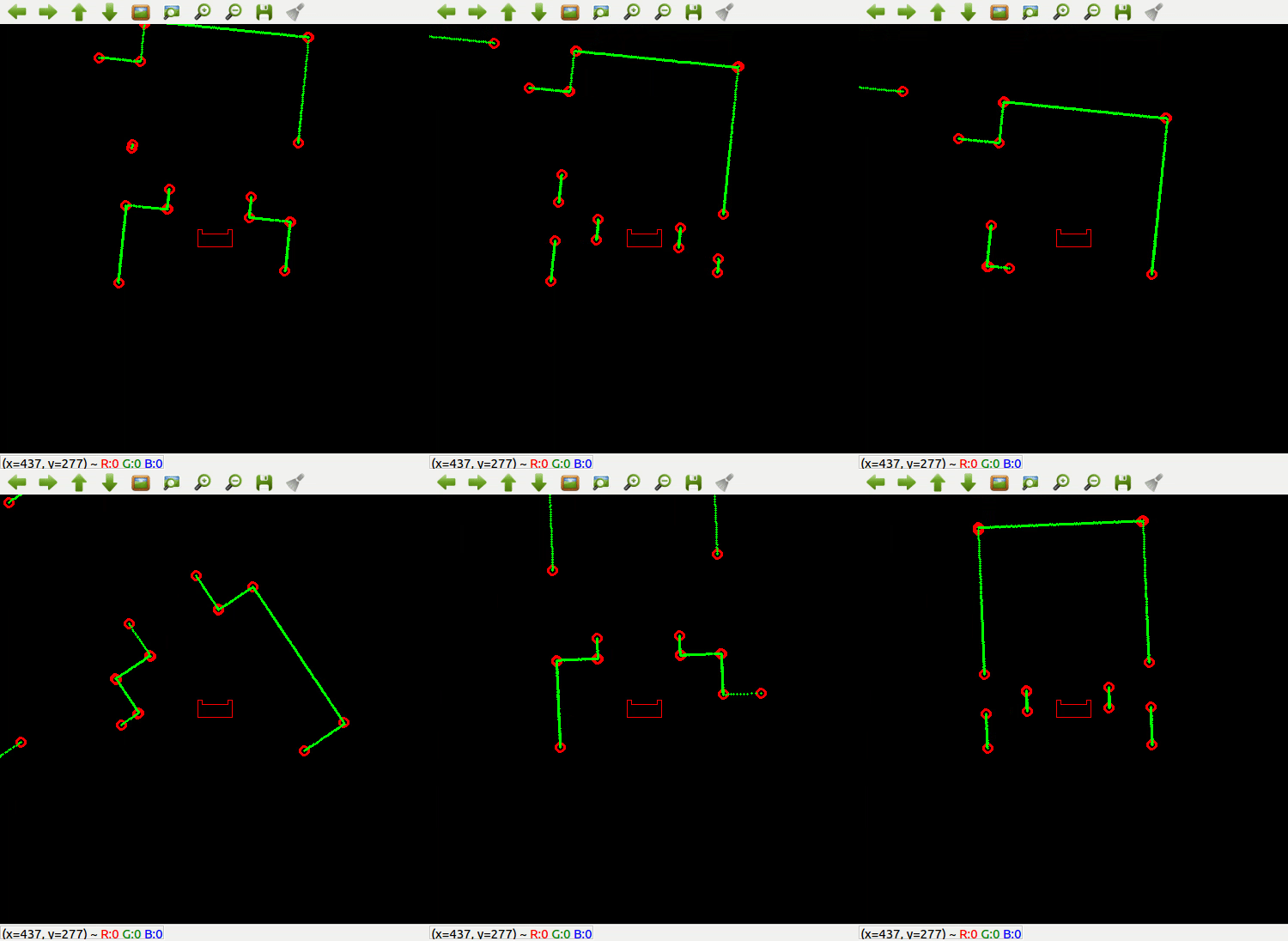
The algorithm starts by considering all 1000 points as a prospective line segment with the first and last points as the start and end. Then for every point in between it determines the orthogonal distance to a line spanned between the end points. While iterating the point with the largest distance is remembered. If the farthest point is closer to the line than a certain threshold a definitive segment is found and added to the list of segments. If the point is farther away than the threshold it is used to split the prospective segment.

The new prospective segment has the same first point, the last point has been changed to the farthest point found before. The algorithm iteratively splits the prospective segments this way until a valid one is found. Then a new prospective segment is considered. The first point of this is the one at the end of the previous segment, plus one. Segments do not share points, this is done to account for gaps in the walls. The last point of this segment is again the 1000th point.

The segmentation algorithm is demonstrated in Figure [segmentation_figure].

The algorithm continues splitting segments and adding them to the list until the end point of a definitive segment is the 1000th point. Then the end is reached. The code implementation uses two methods: individualLineSegmentation() receives the start and end points of a prospective segment and determines if it is a valid one, and if it isn’t it returns the point that is farthest from the line. LineSegmentation() receives the output from individualLineSegmentation() saves valid line segments and determines the next prospective line segment.

Line Fitting

The segmentation algorithm only finds the first and last point making up a wall, the measurements for these contain noise. To mitigate that noise a line is fitted through all the points making up the wall segment. This is done using a Total Least Squares regression. This looks at deviations in two directions and fits a line that minimizes the orthogonal distance between the points and the line. Later when filtering the features, the intersection between two lines can be used as a better estimate of the corner position.

During debugging it turned out that an increase in accuracy was not needed and this method was skipped in the end.

Landmark Creation

A struct of landmarks is created that consists of all the points at the ends of the segments.

Corner Detection

Figure ?: The different types of landmarks detected

The landmark matching algorithm used later computes the distance between all detected landmarks and all the landmarks in the hospital map. However, only about half the detected landmarks denote actual corners. In general PICO sees between two and around 15 segments, 30 landmarks. Excluding moving objects, the hospital has 115 landmark corners. With n detected landmarks and m map landmarks, matching is an O(n*m) operation. This corner detection is an O(n) operations that halves the number of landmarks passed on.

There are four types of landmarks that PICO can see:

1. A corner that is seen in its entirety.

   Here two segments meet and two landmarks are close together. Only one landmark is needed and the midpoint between the landmarks is saved.

2. A corner that is seen from one side and inferred.
3. The end of a wall’s observation caused by occlusion.

   These two exist when one wall is in front of another. As seen from PICO there are two landmarks close to each other in angle but far apart in range. The landmark farthest from PICO is not a corner, PICO just doesn’t see the end of the wall. The closest landmark is an actual corner and is saved.

4. The end of a wall’s observation caused by PICO’s blind spot.

   The first and last landmarks are not corners but again the end of PICO’s observation of a wall.

These different detected landmarks are illustrated in Figure ?.

The method used, computeVisibleLandmarks(), iterates with a step size of two over the landmarks and compares them to the next in the list. This way only sequential landmarks belonging to different segments are compared. The comparison checks if the pair of landmarks are close together, if so it indicates they are type (1) and adds the midpoint between the two to a new list of landmarks. If not it checks if the pair makes a set type (2) and type (3), if so it adds the closest one to the list. The first and last landmarks are always skipped. This method is not essential for functioning, it only filters the landmarks to make another computation faster. Due to some debugging problems this method was skipped over in the end.

Corner Identification

All the landmarks in the hospital map have a numbered ID. The goal of the method labelLandmarkIDMatched() is for every detected landmark to find the map landmark that corresponds to it and copy it’s ID. The method iterates over the detected landmarks. For each detected landmark it then iterates over all map landmarks and computes the distance between the two. If that distance is smaller than a certain threshold a match is made

The coordinates of the detected landmarks are all from the point of view of PICO. With the method transformationLoToGo() they are transformed into the coordinate system of the map using the latest estimate of PICO’s position and rotation.

Costmap

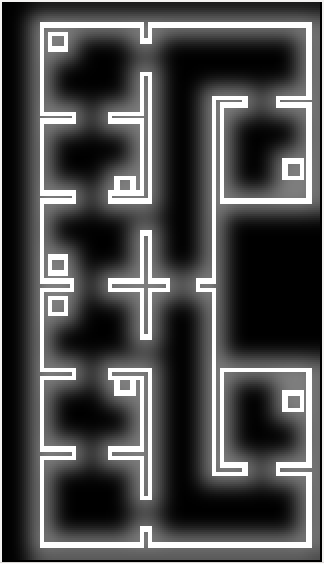
A costmap is made which can be used by the A* pathfinding algorithm to generate a proper path. Here, the white color represents a wall where the PICO cannot go through, and black is the space the PICO can move freely. The blurriness of the white represents the cost of the map. The sharper the white color, the higher the cost.

Closed door detection

The dynamic and static changes that occur in the hospital environment needs to be captured on the global map. A closed-door is one of those changes. Detecting this change is needed since driving through a door is not desirable. Therefore an algorithm to detect a closed-door is implemented.

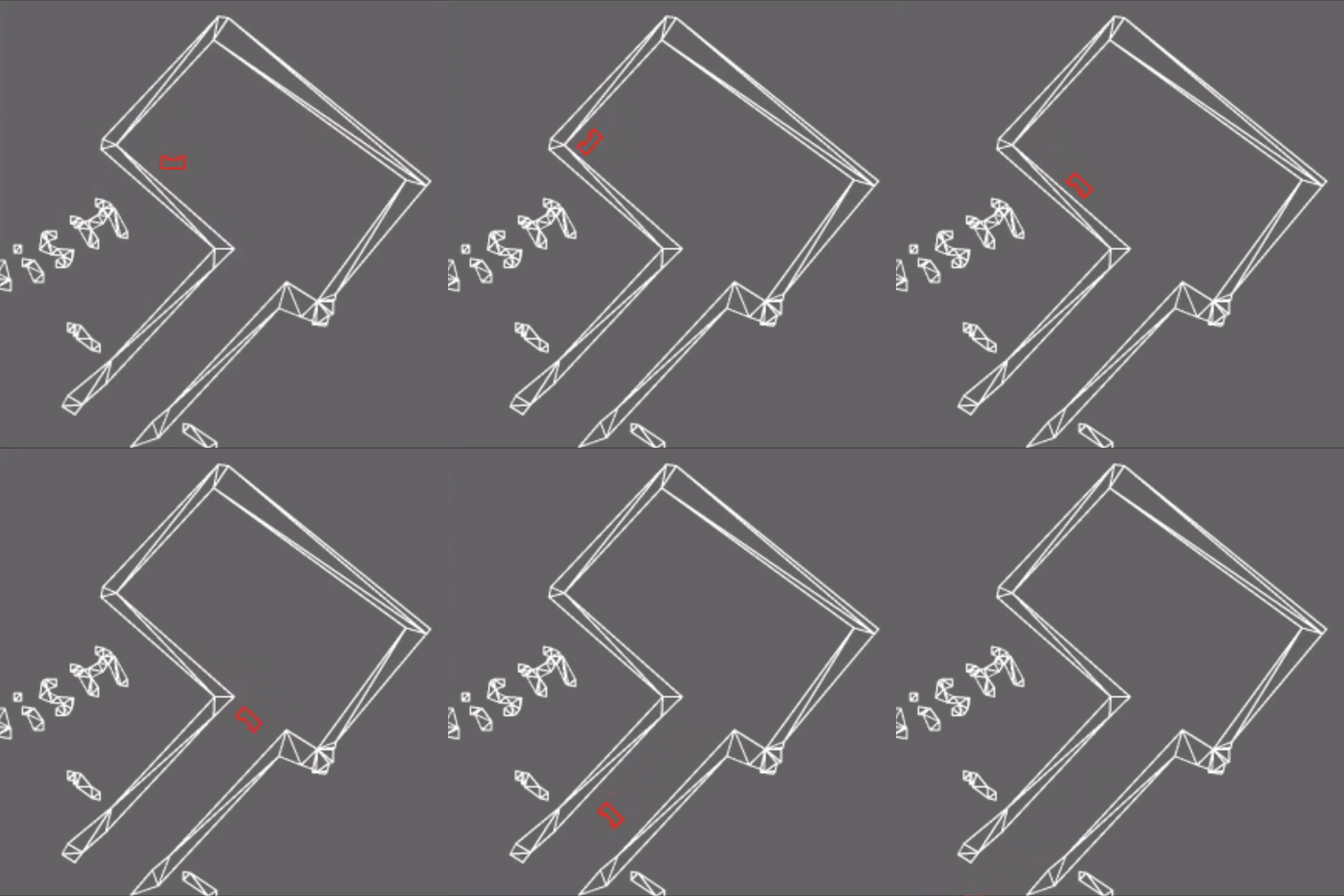
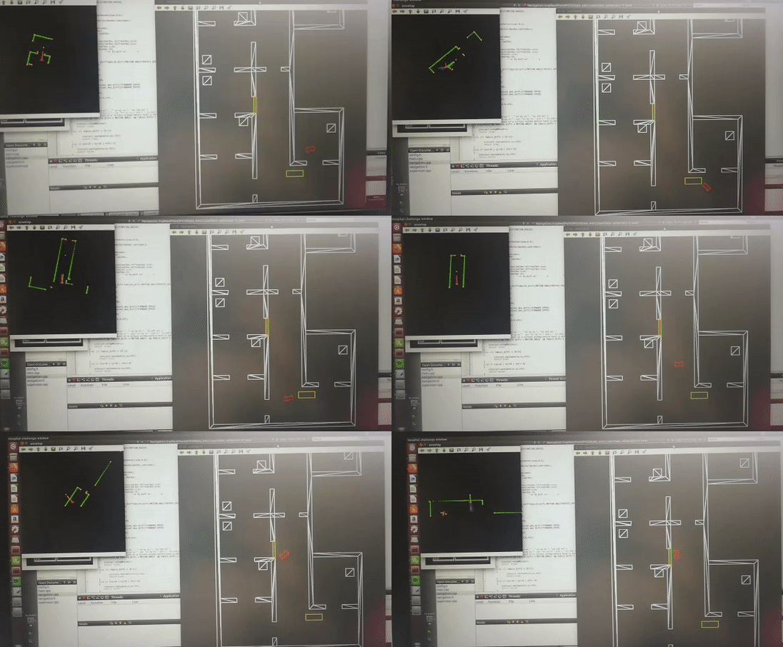
The algorithm is called when the desired velocity vector and the contrary vector, based on the local potential field, results in vector with a near-zero amplitude. This implies that the PICO is positioned in front of a door, which will trigger the door detection. At the start of the program, a map is made on the basis of a JSON file. On top of the labeling of the different landmarks and grouping some of them to form a cabinet, some of them are grouped to form a doorway. Since the position of the robot is known when the door detection algorithm is triggered, the vector of the current position to each of the doorways is calculated. The smallest vector is the doorway that is in front of the PICO. Adding this so-called wall to the vector<Wall> variable will result in adding this wall to the global map. Due to this change, the cost map is updated, which will result in a different A* path. In this way, the closed-door is mapped on the global map. The following figure shows the visuvalisation of the current envelop when a closed door is detected.

Visualization

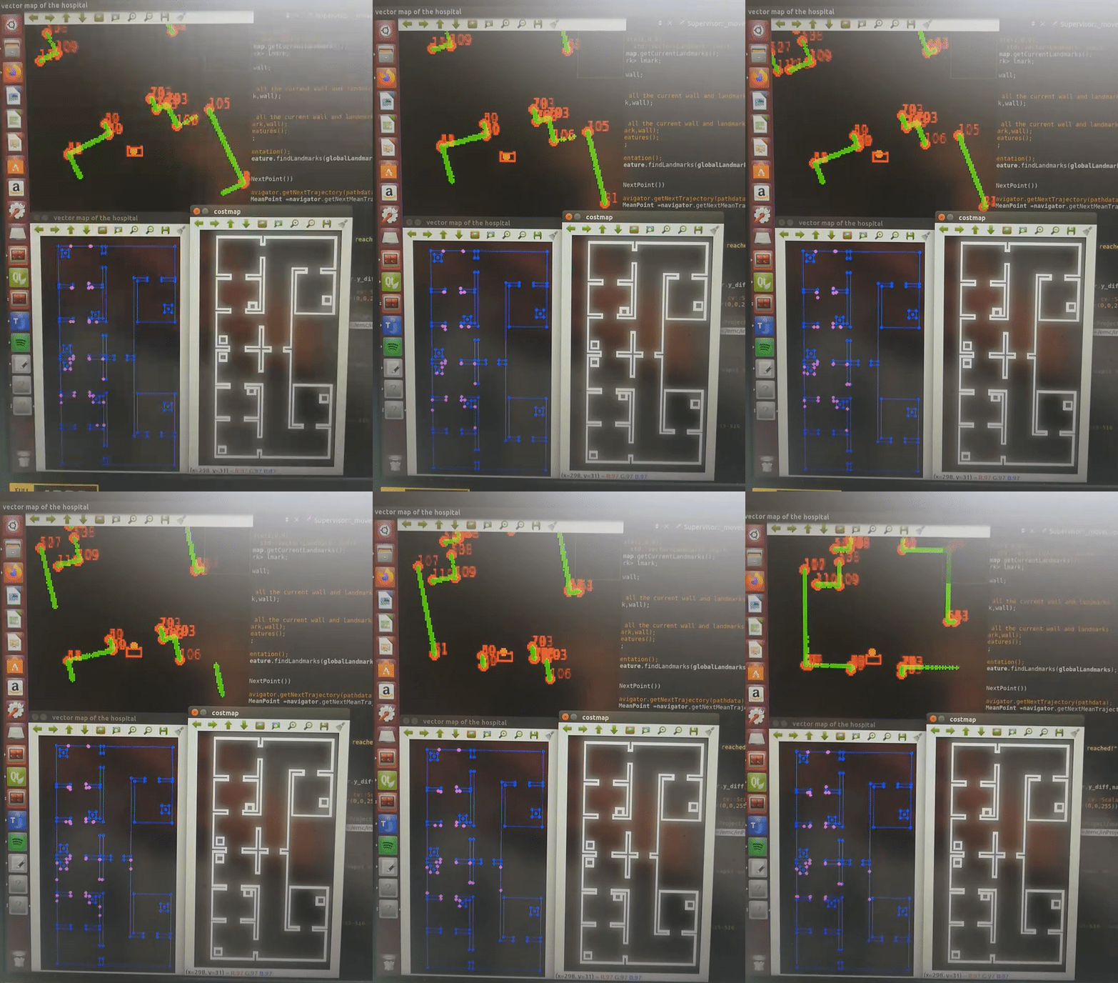
The visualization of the different algorithms is used as a way to check the correctness of the outcome. In total there are three different visualizations, the global map, a costmap of the global map, and the current envelope. The global map is used to check if the robot is correctly orientated. This is done by plotting the seen landmarks in the current envelope on top of the global map. If the local landmarks overlap with the global landmarks, it implies that the robot is correctly orientated. The costmap functions as a basis for the A* algorithm. If the costmap is not correctly defined the A* algorithm will not function as desired or not at all. The costmap is a blurred and tiled version of the global map. Convolution with a gaussian kernel is used to blur the global map, which leads to a valley like distribution in a room. This distribution is desired since this will lead with the A* to a path that goes straight through the middle of a room or hallway. The envelope shows the current laser data with the labeled landmarks from the feature detection. The labeling of the landmarks is checked via this visualization and is shown in the following video.

SLAM

The chosen algorithm for localizing PICO and updating the map with real-world information is fastSLAM2, with the actual implementation largely supported by online lectures and research by Cyrill Stachniss.

The core idea of fastSLAM (especially in its comparison to normal Extended Kalman Filter (EKF) Particle Filter SLAM approaches) is the concept that the relationship between a robot's motion and sensors, and the outside world, is such that given a perfect model, landmarks will always be in the same position. In a more reduced form, using a particle filter to sample the robot's path, this relationship still holds, allowing one to model the outside world as a list of landmarks with a much more static nature than an ever growing hypothetical map of the outside world (which is what normal EKF filters do). Due to this, the measurement covariance element of a single landmark is nothing more than a 2x2 matrix, which, given that it has to be inverted and the most efficient inversion algorithm is O(n3), is a very big deal.

The core idea of fastSLAM2 is to patch a hole in fastSLAM1 where information is lost. Specifically, in the part of the algorithm that is described as 'sampling the pose' - making a prediction, for a particle, of the robot state in the next measurement iteration - fastSLAM2 does not make use of that iteration's measurements. However, by nature of the above relationship, measurements and odometry data are almost equivalently tied to the robot's behaviour. As such, fastSLAM2 includes measurement data when it predicts a robot's state, which, as the paper linked above explains, dramatically improves performance of the algorithm.

Map Updating

Navigation

test test test

This section covers the system functionalities responsible for (intelligent) navigation. All functions here have read access to the world model’s internal map and LRF envelope. The navigation can be split into two parts: pathfinding and path movement.

Path Finding

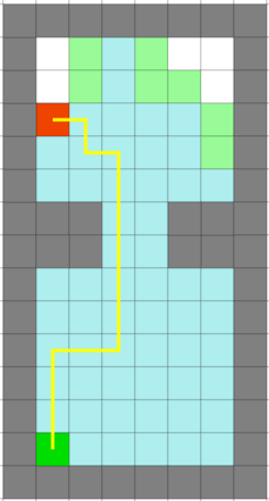
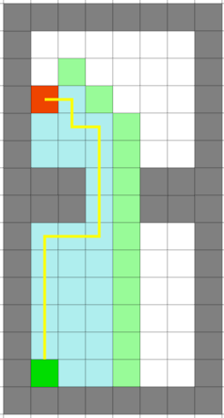
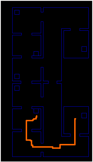
For pathfinding, A* is chosen. A* is a pathfinding algorithm based and built on Dijkstra's Algorithm. Dijkstra's Algorithm looks at every available cell all around the start point, until it reaches the goal. This algorithm uses a costmap to find a proper and efficient path. A* has the same function as Dijsktra, but is smarter, and attaches more value to the cells towards the goal. Because of this, A* needs fewer iterations and is faster. This difference can be seen in the images below, where Dijkstra's algorithm is in the left figure and A* in the right figure. The difference is even more noticeable as the map gets bigger.

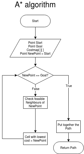
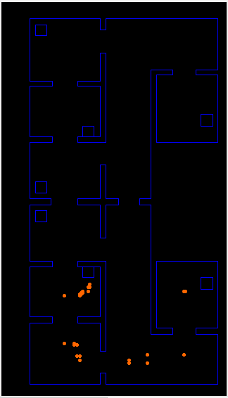
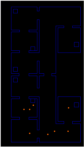
And thus an A* algorithm is made, where the working of the algorithm is explained in the flowchart on the right. A reduction path function is added, which takes the output path of the A* pathfinding function, and removes all of the points which are in the same direction. This ensures that only the important points which needs to be reached are left. Also there is a option in the reduction path function to cluster points which are closely together. With the local potential field (which is further explained in Path Movement) the PICO can move safely even if some points are clustered together. These clustering of points are displayed in the image below, where the first picture displays all of the point returned by the A* algorithm, and thus it got a huge amount of point close to each other. The second image only displays the last point of the same direction of a path. The third image reduces the path even more by clustering point in a specific range.

Path Movement

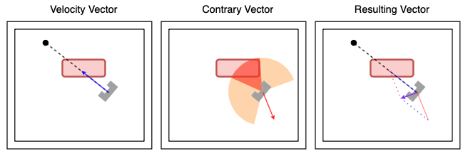
Path movement translates the points of the trajectory of the A* algorithm to a vector of necessary x and y speed values for the PICO robot to follow the trajectory. To make the path movement smoother, and as security for the PICO, a local potential field is used. Based on the objects or walls in a defined range, the PICO generates a contrary vector. The velocity vector and contrary vector together creates a resulting vector, which determines the actual movement direction of the PICO. When the PICO is in a given range of the point it needs to reach, the pico goes to the next point in the path vector, which is put together by the A* pathfinding function.

List of Meetings

	Date/Time	Roles
Meeting 1	01-05-2020 11:00	Chairman: Bas Secretary: Max
Meeting 2	04-05-2020 11:00	-
Meeting 3	08-05-2020 11:00	Chairman: Max Secretary: Dominic
Meeting 4	11-05-2020 10:00	-
Meeting 5	12-05-2020 10:00	-
Meeting 6	15-05-2020 11:00	Chairman: Dominic Secretary: Roel
Meeting 7	18-05-2020 11:00	-
Meeting 8	22-05-2020 11:00	Chairman: Roel Secretary: Rob
Meeting 9	27-05-2020 15:00	-
Meeting 10	29-05-2020 11:00	Chairman: Rob Secretary: Ananth
Meeting 11	02-06-2020 11:00	-
Meeting 12	04-06-2020 11:00	Chairman: Ananth Secretary: Bas

Links

These will probably be invite-based but a backup link could be useful.

Gitlab: https://gitlab.tue.nl/MRC2020/group4

Overleaf design document: https://www.overleaf.com/project/5eabeda72b3e4100010f8b40

Sharepoint: https://tuenl-my.sharepoint.com/:f:/r/personal/r_konings_student_tue_nl/Documents/4SC020%20EMC?csf=1&web=1&e=g6PXRQ

Deliverables

• Design Document
• https://youtu.be/PsSNIyCPNps?t=1630