MRC/Tutorials/Setting up the PICO simulator: Difference between revisions
No edit summary |
|||
| (5 intermediate revisions by 4 users not shown) | |||
| Line 1: | Line 1: | ||
= | = Introduction = | ||
During the course, we have 10 large groups and only one robot, so test time on the robot is scarce. Fortunately, we have a virtual (software) representation of the robot that can be used to simulate the robot. At the moment it: | |||
* Simulates the movement of the robot | |||
* The laser data of the robot, created by the virtual environment | |||
* Provide a simple visualization | |||
This should already be enough to get you started, and more will be added later (odometry, moving doors, better dynamics, etc). | |||
= Updating the simulator = | |||
Before you start working with the simulator, make sure you have our latest version by running | |||
<pre> | <pre> | ||
emc-update | |||
</pre> | |||
This will download the latest changes and compile the updated software (framework and simulator). I will notify you when I made changes to the software such that you can run the updater, but feel free to run the command whenever you want. | |||
= | = Starting the simulator = | ||
As was already stated before, we will not be using ROS in this course, unless you really want to use it yourself. However, secretly the provided tools are build on top of that; the inter-process communication to be more specific. Don't worry about it too much. The only thing you need to know is that before running the simulator or your software, you need to create a ''roscore''. Simply open a terminal an run: | |||
<pre> | |||
roscore | |||
</pre> | |||
and keep it running. This allows processes to 'find' each other and communicate. For example, the software abstraction layer we provide 'talks' to the simulator through this roscore. | |||
Enough about ROS, let's start the simulator! Open a terminal and run | |||
<pre> | |||
emc-sim | |||
</pre> | |||
That's it! What you will see, is a visualization of the virtual environment (the white lines are walls) and a top-down view of the robot (the red lines). | |||
= Controlling the robot = | |||
Now, as you can see, not much is happening. The robot is standing still in a static environment. Let's change that! A first simple way to test the simulator is by controlling the robot using your keyboard. Just run: | |||
<pre> | |||
pico-teleop | |||
</pre> | |||
and you will be able to control the robot using the ''numpad'' keys. You can rotate the robot using '/' and '*'. | |||
= Visualization = | |||
As you already noticed, the simulator pops up a visualization windows showing the robot in the virtual world. This shows how the world ''is'' (at least in simulation...). It is also very interesting to know how to robot ''perceives'' the world through its sensors. Note that this is a big difference! We also created a visualization for that. Just run | |||
<pre> | |||
emc-viz | |||
</pre> | |||
You will again see the robot footprint displayed in red. However, the walls are gone and replaced by the actual (simulated) sensor data from the robot (the green dots). The laser data is actually represented in polar coordinates (remember, the LRF is a laser with a rotating mirror, so what it will return are angles and distances) but the visualization 'projects' them back to world coordinates. See how the laser data changes even if the robot is standing still: this is the simulated noise added to the data. | |||
Try driving the robot around using 'pico-teleop' and notice how the laser data changes, and how it differs from the actual virtual world. | |||
= Stopping the simulator and visualization = | |||
You can stop the simulator and visualization by pressing ''ctrl-C'' in the terminal. | |||
= Loading a custom heightmap = | |||
By default, the simulator loads a pretty ugly maze. Fortunately, you can change the simulation environment very easily! You just have to create a heightmap: an image that specifies for each pixel how 'high' the world has to be at that point. Since the laser only scans at one height, we can use two extremes here: flat (ground level) or high enough to be detected by the laser. | |||
To create an image, simply open your favourite image editor and create a black-and-white image. If you don't know how to create an image, have a look at the section below. White corresponds to the floor, black to the walls (i.e., which will be detected by the laser). You have to keep the following things in mind: | |||
* The simulator converts the pixels to world coordinates. Each pixel corresponds to a block of 2.5 by 2.5 cm, or in other words, 40 pixels correspond to 1 meter. | |||
* The robot always starts in the center of the image. So, if you want to robot to start at the edge of your maze / corridor, just create a bigger image and move the black pixels to the upper part of the image. | |||
* You'll get the best result if the lines drawn are at least 2 pixels wide | |||
* Store your image lossless, ''i.e.'' using the ''png'' format (which is recommended by the way!), instead of the ''jpg'' format. | |||
* Make sure your heightmap images always have a border of white pixels, ''i.e.'' there should '''not''' be any non-white pixels at the borders of your image | |||
Once you have created an image, simply run the simulator and provide the image file as argument: | |||
<pre> | |||
emc-sim --map <YOUR_IMAGE_FILE>.png | |||
</pre> | |||
That's it! | |||
== Create a heigthmap image == | |||
There are many linux applications that you use to create images. We suggest using Gimp, an open-source alternative to Photoshop. Although it might be a bit overkill to use for our application, it has great support and the thing we want to do (draw black lines on a white background) isn't hard. To install Gimp, run: | |||
<pre> | |||
- | sudo apt-get install gimp | ||
</pre> | |||
And run it using: | |||
<pre> | |||
gimp | |||
</pre> | |||
Then to create a simple image: | |||
* Select ''File'' -> ''New'' (or ''ctrl-N'') | |||
* Specify the size of your image. Remember, 40 pixels = 1 meter, and the robot starts in the center | |||
* Select the ''Pencil Tool'' from the left pane. | |||
* Set the pencil size in the lower left pane to something sensible, ''e.g.'' 2 pixels | |||
Now, if you click left on the image, a dot is drawn, but we want lines! To draw a line: | |||
* left click, ''then'' hold ''shift'', ''then'' left click again. | |||
* While holding the ''shift'' button, you can click more times to create a sequence of lines | |||
* To create nice, axis-aligned lines, also hold ''ctrl'' | |||
That's | There is two types of saving in Gimp. The first one is the using ''File'' -> ''Save''. However, this will only generate an ''xcf''-file, something that can only be read by Gimp. Instead, you should use the ''File'' -> ''Export'' option: | ||
* ''File'' -> ''Export'' | |||
* Provide a name for your file. If you put '.png' as extension, it will be saved as png | |||
* Use the default ''png'' export settings | |||
That's it! | |||
== Adding clutter objects and simulating wheelslip == | |||
In the real world, the odometry that is returned by the robot is not perfect and will have a certain amount of drift. | |||
Furthermore, the internal representation of the map never matches 100% with the real world. | |||
To add these discrepancies to the simulator (which are disabled by default), a JSON config file can be supplied. | |||
In this file it is easy to specify an array of objects that will be added to the world and to enable wheelslip. | |||
An example of this file is shown below: | |||
<pre> | |||
{ | |||
"uncertain_odom":true, | |||
"show_full_map":true, | |||
"objects":[ | |||
{ | |||
"length": 1.0, | |||
"width": 1.0, | |||
"trigger_radius": 1.0, | |||
"repeat": false, | |||
"velocity": 0.6, | |||
"init_pose": [-1.0, 0.0, 0.0], | |||
"final_pose": [-1.0, -2.0, 0.0] | |||
}, | |||
{ | |||
"length": 0.2, | |||
"width": 0.4, | |||
"trigger_radius": 1.0, | |||
"repeat": true, | |||
"velocity": 1.3, | |||
"init_pose": [1.4, 0.0, 0.0], | |||
"final_pose": [1.4, 1.0, 0.0] | |||
} | |||
] | |||
} | |||
</pre> | |||
In this file, the "uncertain_odom" is enabled, and the robot is visualized in the static map by setting "show_full_map". | |||
Furthermore, two objects are added, which will start to move from their "init_pose" to (approximately) their "final_pose", supplied in (x,y,theta) coordinates. | |||
This movement is triggered when pico comes within the "trigger_radius" of the object, and the second object will keep repeating its movement. | |||
To supply such a file to the simulator, use the following argument: | |||
<pre> | |||
emc-sim --config <YOUR_CONFIG_FILE>.json | |||
</pre> | |||
The wheelslip is simulated by random sampling a slip factor every few seconds, making the simulator stochastic. | |||
The result is that, just like with the real robot, no two trials will result in exactly the same robot position and odometry. | |||
== Adding doors (not needed for this year)== | |||
The real maze will contain a door that the robot needs to open. The simulator is capable of simulating these doors, such that you can test your software before it gets real! To add doors to the simulated world, simply edit your heightmap and add ''grey'' lines to it. To be specific: | |||
* The door should be a straight line (but not necessarily axis-aligned), with a minimum thickness of 2 pixels. To be more specific, all pixels in the door line should be connected | |||
* The average RGB value should be between 50 and 205 (on a scale of 0-255). So for example, the RGB value (100, 100, 100) is a door, while (20, 20, 20) is a wall (and (255, 255, 255) is open space). | |||
* You can have multiple doors in your world. However, make sure that they are always separated by at least one pixel. ''Remember that there will only be one door, i.e, one sliding block, in the final maze'', but the possibility of having multiple doors to test with in simulation might be nice. | |||
* You can experiment with the direction in which it slides open. Darker lines (RGB values below 128) will open in a different direction than lighter lines (RGB values above 128). | |||
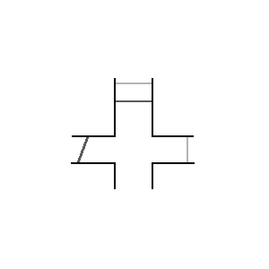
An example: [[Media:Emc2015-heightmap-example.png | Height Map]]. Note that doors as skewed as the left one in the example will not occur in the final maze (but are allowed in the simulation, for you to test with). | |||
The doors should be visible as green blocks in the simulator. Now, you can use the ''emc::IO'' object from your code to open these doors (but only if you are standing in front): | |||
<pre> | |||
// ... Make sure robot is in front of a possible door | |||
// ... Make sure robot is standing still | |||
io.sendRequestOpenDoor(); | |||
</pre> | |||
Latest revision as of 12:09, 9 April 2020
Introduction
During the course, we have 10 large groups and only one robot, so test time on the robot is scarce. Fortunately, we have a virtual (software) representation of the robot that can be used to simulate the robot. At the moment it:
- Simulates the movement of the robot
- The laser data of the robot, created by the virtual environment
- Provide a simple visualization
This should already be enough to get you started, and more will be added later (odometry, moving doors, better dynamics, etc).
Updating the simulator
Before you start working with the simulator, make sure you have our latest version by running
emc-update
This will download the latest changes and compile the updated software (framework and simulator). I will notify you when I made changes to the software such that you can run the updater, but feel free to run the command whenever you want.
Starting the simulator
As was already stated before, we will not be using ROS in this course, unless you really want to use it yourself. However, secretly the provided tools are build on top of that; the inter-process communication to be more specific. Don't worry about it too much. The only thing you need to know is that before running the simulator or your software, you need to create a roscore. Simply open a terminal an run:
roscore
and keep it running. This allows processes to 'find' each other and communicate. For example, the software abstraction layer we provide 'talks' to the simulator through this roscore.
Enough about ROS, let's start the simulator! Open a terminal and run
emc-sim
That's it! What you will see, is a visualization of the virtual environment (the white lines are walls) and a top-down view of the robot (the red lines).
Controlling the robot
Now, as you can see, not much is happening. The robot is standing still in a static environment. Let's change that! A first simple way to test the simulator is by controlling the robot using your keyboard. Just run:
pico-teleop
and you will be able to control the robot using the numpad keys. You can rotate the robot using '/' and '*'.
Visualization
As you already noticed, the simulator pops up a visualization windows showing the robot in the virtual world. This shows how the world is (at least in simulation...). It is also very interesting to know how to robot perceives the world through its sensors. Note that this is a big difference! We also created a visualization for that. Just run
emc-viz
You will again see the robot footprint displayed in red. However, the walls are gone and replaced by the actual (simulated) sensor data from the robot (the green dots). The laser data is actually represented in polar coordinates (remember, the LRF is a laser with a rotating mirror, so what it will return are angles and distances) but the visualization 'projects' them back to world coordinates. See how the laser data changes even if the robot is standing still: this is the simulated noise added to the data.
Try driving the robot around using 'pico-teleop' and notice how the laser data changes, and how it differs from the actual virtual world.
Stopping the simulator and visualization
You can stop the simulator and visualization by pressing ctrl-C in the terminal.
Loading a custom heightmap
By default, the simulator loads a pretty ugly maze. Fortunately, you can change the simulation environment very easily! You just have to create a heightmap: an image that specifies for each pixel how 'high' the world has to be at that point. Since the laser only scans at one height, we can use two extremes here: flat (ground level) or high enough to be detected by the laser.
To create an image, simply open your favourite image editor and create a black-and-white image. If you don't know how to create an image, have a look at the section below. White corresponds to the floor, black to the walls (i.e., which will be detected by the laser). You have to keep the following things in mind:
- The simulator converts the pixels to world coordinates. Each pixel corresponds to a block of 2.5 by 2.5 cm, or in other words, 40 pixels correspond to 1 meter.
- The robot always starts in the center of the image. So, if you want to robot to start at the edge of your maze / corridor, just create a bigger image and move the black pixels to the upper part of the image.
- You'll get the best result if the lines drawn are at least 2 pixels wide
- Store your image lossless, i.e. using the png format (which is recommended by the way!), instead of the jpg format.
- Make sure your heightmap images always have a border of white pixels, i.e. there should not be any non-white pixels at the borders of your image
Once you have created an image, simply run the simulator and provide the image file as argument:
emc-sim --map <YOUR_IMAGE_FILE>.png
That's it!
Create a heigthmap image
There are many linux applications that you use to create images. We suggest using Gimp, an open-source alternative to Photoshop. Although it might be a bit overkill to use for our application, it has great support and the thing we want to do (draw black lines on a white background) isn't hard. To install Gimp, run:
sudo apt-get install gimp
And run it using:
gimp
Then to create a simple image:
- Select File -> New (or ctrl-N)
- Specify the size of your image. Remember, 40 pixels = 1 meter, and the robot starts in the center
- Select the Pencil Tool from the left pane.
- Set the pencil size in the lower left pane to something sensible, e.g. 2 pixels
Now, if you click left on the image, a dot is drawn, but we want lines! To draw a line:
- left click, then hold shift, then left click again.
- While holding the shift button, you can click more times to create a sequence of lines
- To create nice, axis-aligned lines, also hold ctrl
There is two types of saving in Gimp. The first one is the using File -> Save. However, this will only generate an xcf-file, something that can only be read by Gimp. Instead, you should use the File -> Export option:
- File -> Export
- Provide a name for your file. If you put '.png' as extension, it will be saved as png
- Use the default png export settings
That's it!
Adding clutter objects and simulating wheelslip
In the real world, the odometry that is returned by the robot is not perfect and will have a certain amount of drift. Furthermore, the internal representation of the map never matches 100% with the real world. To add these discrepancies to the simulator (which are disabled by default), a JSON config file can be supplied. In this file it is easy to specify an array of objects that will be added to the world and to enable wheelslip. An example of this file is shown below:
{
  "uncertain_odom":true,
  "show_full_map":true,
  "objects":[
    {
      "length": 1.0,
      "width": 1.0,
      "trigger_radius": 1.0,
      "repeat": false,
      "velocity": 0.6,
      "init_pose": [-1.0, 0.0, 0.0],
      "final_pose": [-1.0, -2.0, 0.0]
    },
    {
      "length": 0.2,
      "width": 0.4,
      "trigger_radius": 1.0,
      "repeat": true,
      "velocity": 1.3,
      "init_pose": [1.4, 0.0, 0.0],
      "final_pose": [1.4, 1.0, 0.0]
    }
  ]
}
In this file, the "uncertain_odom" is enabled, and the robot is visualized in the static map by setting "show_full_map". Furthermore, two objects are added, which will start to move from their "init_pose" to (approximately) their "final_pose", supplied in (x,y,theta) coordinates. This movement is triggered when pico comes within the "trigger_radius" of the object, and the second object will keep repeating its movement. To supply such a file to the simulator, use the following argument:
emc-sim --config <YOUR_CONFIG_FILE>.json
The wheelslip is simulated by random sampling a slip factor every few seconds, making the simulator stochastic. The result is that, just like with the real robot, no two trials will result in exactly the same robot position and odometry.
Adding doors (not needed for this year)
The real maze will contain a door that the robot needs to open. The simulator is capable of simulating these doors, such that you can test your software before it gets real! To add doors to the simulated world, simply edit your heightmap and add grey lines to it. To be specific:
- The door should be a straight line (but not necessarily axis-aligned), with a minimum thickness of 2 pixels. To be more specific, all pixels in the door line should be connected
- The average RGB value should be between 50 and 205 (on a scale of 0-255). So for example, the RGB value (100, 100, 100) is a door, while (20, 20, 20) is a wall (and (255, 255, 255) is open space).
- You can have multiple doors in your world. However, make sure that they are always separated by at least one pixel. Remember that there will only be one door, i.e, one sliding block, in the final maze, but the possibility of having multiple doors to test with in simulation might be nice.
- You can experiment with the direction in which it slides open. Darker lines (RGB values below 128) will open in a different direction than lighter lines (RGB values above 128).
An example: Height Map. Note that doors as skewed as the left one in the example will not occur in the final maze (but are allowed in the simulation, for you to test with).
The doors should be visible as green blocks in the simulator. Now, you can use the emc::IO object from your code to open these doors (but only if you are standing in front):
// ... Make sure robot is in front of a possible door
// ... Make sure robot is standing still

io.sendRequestOpenDoor();