Embedded Motion Control 2018 Group 7

Group Members

TU/e Number	Name	E-mail
0833049	Sam Roovers	s dot roovers at student dot tue dot nl
0886654	Siebrand Keja	s dot c dot keja at student dot tue dot nl
1022624	Milan Haverlag	m dot a dot haverlag at student dot tue dot nl
1279637	Piyush George Alexander	p dot g dot alexander at student dot tue dot nl

Initial Design

The Initial Design document can be found here : File:Emc-designrequirements.pdf

Escape room competition

To escape the room, PICO will first scan its surroundings. By the use of a corner detection program the exit is determined from two laser sets (from the front and back). PICO aligns with the angle at which the exit is detected and will drive forward. A potential field must make sure that PICO does not hit any walls.

Simulation for the Escape room challenge is shown below.

Figure 1 Animation of the Escape room challenge

Exit detection

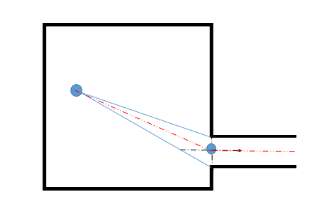
For detecting the exit, the range from the laser data was considered. PICO does a 360 degree scan and detects an exit point based on distance criteria, i.e. if the distance between consecutive sections is within the exit door tolerance ( 0.5-1 m). After detecting the two points, it searches for the point right in the middle of the detected points, which would be a waypoint for PICO to drive to, followed by which it would drive till the exit is reached.

Figure 2 Exit detection

Potential field method

In order to prevent PICO from crashing into the walls, obstacle avoidance is needed. For this it is chosen to implement potential field method. The potential field method works by combining a attractive force towards a desired set-point with repulsive forces generated from obstacles.

The Attractive force is calculated from the distance between the robot and the set-point. [math]\displaystyle{ r_{att} = \sqrt{(x_{set}-x_{PICO})^2+(y_{set}-y_{PICO})^2} }[/math] and the angle: [math]\displaystyle{ \alpha_{att} = tan(\frac{x_{set}-x_{PICO}}{y_{set}-y_{PICO}}) }[/math]

The attractive force is calculated using a proportional controller:

[math]\displaystyle{ F_{att} = r_{att}*K_{att} }[/math]

The repulsive forces are calculated by taking the inverse of the distance to the wall measured with the laser range finder with the following formula: [math]\displaystyle{ r_{rep}(i) = \sqrt{(x_{wall}(i)-x_{PICO})^2+(y_{wall}(i)-y_{PICO})^2} }[/math] [math]\displaystyle{ F_{rep}(i) = \frac{K_{rep}}{r_{rep}(i)^3} }[/math]

The attractive and repulsive forces are then split in their x and y parts. Their respective x an y parts are then added together:

[math]\displaystyle{ F_{tot}(x) = F_{att}(x) + \sum{F_{rep}(i)(x)} }[/math] [math]\displaystyle{ F_{tot}(y) = F_{att}(y) + \sum{F_{rep}(i)(y)} }[/math]

These Forces are then used to determine where PICO should drive to.

Shortcommings

Due to time constraints the following features are not implemented which would have made the escape room routine a lot better.

• the positioning of a waypoint in front of the exit with enough clearing from the walls to drive to.
• alignment with the corridor after the waypoint has been reached.

Hospital challenge

Main Loop

Scanning the hospital map

The first part of the challenge consists of mapping the hospital. The program to do this consists of the following steps

Step 1: Pico rotates 360 degrees at its starting position to start creating a map of the hallway. The program calculates the end of the hallway using the furthest set of corners that it can find. A way-point is place half a meter from the end and Pico drives to that way-point. When Pico has arrived at the way-point, it starts rotating 360 degrees again completing the map of the hallway.

Step 2: The program tries to find the doors by looking at corner points found while scanning the hallway. Way-points are then placed in front and behind the center point of the found exits. The way-points that are placed behind the exit are each given a new room number. The created way-points are considered connected with each other, meaning that the robot can use them to drive to another room.

Step 3: The program checks which way-point is closest. If no way-point can be found that has not already been used, Pico will check which room it is in at that moment. If Pico is in the hallway, Pico will go back to its initial location and go to the parking program. If Pico is not in the hallway, it will check from which way-point it entered the room and go back through that way-point. If a unused way-point is found Pico drives towards that way-point. When Pico arrives at the closest way-point,it then drives to the way-point thats connected to it. The program starts rotating 360 degrees again, adding the room to the exiting map of the hallway.

Step: 4 The program again tries to find the doors by looking at corner points found while scanning the new room. Way-points are then placed in front and behind the center point of the found exits. The way-points that are placed behind the exits are each given a new room number. Steps 2-4 are repeated until no more unused way-points are found in any of the rooms.

Feature Detection

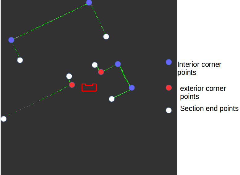
For the detecting the features first it is essential to find out the number of sections in the surrounding. A section comprises a continuous set of data points. A section ends when the distance between consecutive data points exceeds a threshold value. In this case, it is 0.5. In the function that is made, the section details are verified by returning the indexes of the beginning and end section details into separate vectors. The index details are further used to determine the number of sections. The beginning and end details of each section is used in the split and merge algorithm to find the corners and ultimately return a 2 dimensional vector in which each row corresponds to each section and each column has elements which are of a structure type that has the x and y coordinate details, whether itś an intermediate point/ corner and if itś an exit corner or not.

In order to generate the Map, it is essential to detect the features. This is attained using a split and merge algorithm. The basic idea of the split and merge algorithm is as follows if the endpoint and the starting point of the section are known, it fits a line between these two points and evaluates the distance of each point from this line. The point that is at a maximum distance from this line, greater than the threshold set for it being part of a wall, would be marked as corner point1, and a boolean would mark it as false for a corner point( true for intermediate point). If not, it would be identified as a wall. Now the program searches for any more corners between the starting point and the corner point1 and in between the corner point 1 and the exit point. If it finds more corner points it returns the details of these corner points and repeats until only wall segments are identified. For a section, the function ultimately returns the initial point, corner1, corner2 ... corner#n, the endpoint of the section as each row.

Algorithm

The Modified split and merge algorithm works in the following sequence:

• The starting node = Section beginning point, ending node is the section ending point.
• Line is fitted between these points and distance to each point in between is found.
• distance of each point inbetween from the fitted line is determined with the equation given below.

dist = abs( a*x+ b*y + c )/ sqrt( a²+ b² )

a = (yi - ye)/(xi - xe)

b = -1 

c= (xi*ye - xe*yi)/(xi - xe)

• Check is all distances are within the threshhold.( here threshhold was tuned to 0.1 considering the fact that the wall thickness is 20 cm.

 if (distance < threshold )

Return the initial and end point with flag as true indicating that itś a wall. 

else fit lines line between the initial point - cornerpoint found and the exit - corner point and search for more corners. 

If all wall segments are identified with no more corners, return for the current section, the initial point, corner 1, corner 2 ... etc end point in sequence.

goto the next section, follow the same steps until the last section. 

For illustration refer the sequence generated below.

The feature depends on laser data as input, the data on reading the CSV file showed several data points as Nan( not a number). These are eliminated from the section by filtering the laser data.

• Separate structure to characterize the points(Marker Allocation)

Figure 2 Exit detection

Every point that has been detected is a structure of the following form.

• x coordinate
• y coordinate
• bool, true if itś an intermediate point, false if a corner
• bool, true if itś an exit corner

• Characterizing the corners found.

• Identifying the exit points

Test results

show the generated image

Debugging interface

Figure 4 debugging interface

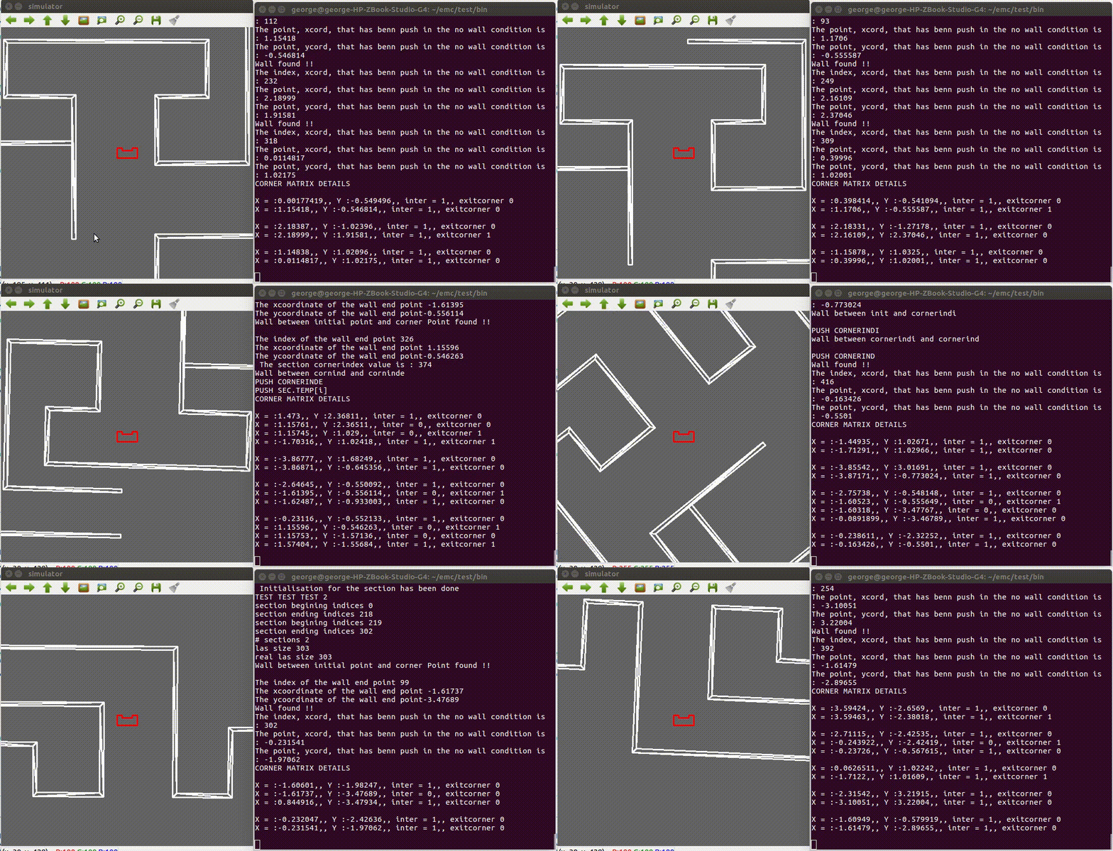
The above interface was used to debug the modified split and merge algorithm. It gives real time values that are detected as corner/ intermediate points and on whether they are exit or not( from the bool flag). As PICO moves through the map it dynamically gives out the point which can be verified from the map used for in the PICO simulator.

Difficulties faced and solutions

• Missing corners case .

• fitted line being parallel case

Localization

The odometry localization present on PICO is only accurate for a short time due to the wheels slipping. In order to improve the accuracy of the localization, laser rangefinder data is combined with the odometry data.

When the robot starts, it scans its surroundings using the laser rangefinder and stores the found wall positions to a world map with its initial position being the center point. At the start of the main loop, the localization algorithm uses the odometry data to determine its approximate position. it the scans its surroundings using the rangefinder. in an area around the approximated position, the algorithm searches for a position where the wall locations found with the laser rangefinder can be best fitted on the world map. The fitting is done by comparing the wall locations with the world map for multiple locations. A Gaussian filter with a 5x5 kernel is used to create a smoother world map to compare to. The location where the best fit can be made is taken as the current position of the robot. The fitted laser rangefinder data is then added to the world model to expand the map.