Embedded Motion Control 2017 Group 4
Initial design report & Final design presentation
File:Final design presentation.pdf
Group 4
| M.R.M. Beurskens | 0843080 |
| N.H.J. Janssen | 0842075 |
| M.C.W. Schouten | 0869793 |
| J.A.E. Verest | 0844791 |
| M.S. de Wildt | 0776941 |
| R.H.M. Winters | 0854048 |
Initial design
Introduction
In this design chapter, the initial design of a maze solving robot is specified in terms of requirements, specifications, components, functions and interfaces. It is implemented on the PICO hardware platform. A task-skill-motion framework is used in order to describe the robot behaviour. This will also be implemented in C++.
Requirements and specifications
PICO is required to autonomously navigate through a maze and find the exit without bumping into any of the walls. A door will be present in the maze, and must be opened by "ringing the bell" in a suitable location whilst standing still. Open spaces might be present, and the walls are approximately axis aligned. The maze might also feature loops. Therefore PICO is required to do the following:
- Recognize walls and corridors in a robust manner. The walls are axis aligned, however not perfectly. PICO should allow for an alignment error. It also has to stay away from the walls with a sufficient margin (e.g. 10 cm between robot and wall). Bumping into a wall will count as a failed attempt.
- Identify possible "door areas" in a robust manner. "The door will be situated at a dead end, a dead end being defined as a piece of wall with minimum length 0.5 meter and maximum length 1.5 meter with side-walls of at least 0.3 meter length". Alignment errors again need to be taken into account.
- Map the maze to determine whether the area has been visited and to build a world model. Odometry and a Laser Range Finder (LRF) are used to build a world map and determine the location in the world. The odometry and LRF data should be synchronized to avoid drift in world location and mapping (SLAM).
- Recognize corners as nodes in order to build an abstract and simplified maze representation consisting of nodes and lines.
- Carry out a maze solving strategy based on its world model and solve and execute corresponding routing. The solving routine and the routing should be able to handle loops and open spaces and are based on the simplified maze representation. This enables more general strategy composition and faster computation.
- Open doors by ringing a bell in the door area. No part of PICO should be located outside the 1.3 meter range of the door and PICO should be standing still whilst ringing the bell. The door opens completely within 5 seconds after PICOs request. Once the door is completely open, PICO needs to pass the open doorway to find the exit of the maze.
- The software should be easy to set up and deploy, i.e. using git pull and with a single executable.
- Clear the maze as soon as possible, with a total available time of seven minutes for two attempts. A maximum speed of 0.5 m/s translational and 1.2 rad/s rotational is given.
- Do not stand still for more than thirty seconds when inside the maze.
Components
PICO features a Laser Range Finder (LRF) to detect surrounding obstacles and wheel encoders to measure odometry data. The wheel base is holonomic, enabling it to turn on the spot and drive in any direction. An emergency button is present on the remote. PICO runs on batteries and should always be charging when not driving around.
The software runs on an Intel i7 processor running Ubuntu 14.04 LTS. The Robotic Operating System (ROS) is used as a framework for PICOs software. However, an intermediate software layer is provided which can be used to access sensor data and actuate the robot. Our own software layer is divided into five main components: actuation, sensing, world model, task manager and skill.
Functions
Configuration file
- Configuration: Defines a number of parameters. This is a header file so no inputs or outputs.
Actuation
- Move: This function calculates the translational velocity in x and y direction and the rotational velocity corresponding to the direction vector and net velocity outputted by the path planning function. The calculated velocities are sent tot the base actuators.
- Input: Direction vector, total velocity, Output: -.
- Stop: Stops the robot by sending the base velocities of magnitude zero.
- Input:-, Output:-.
- Rotate: Rotates the robot 90 or 180 degrees. First checks the robot has enough space to rotate without hitting the wall. If this is not the case, first a call to Move is made to move the robot away from the wall.
- Open door: Makes sure the robot stands still, rings the bell to open the door and waits until the door is opened.
- Input: LRF data, Output: -.
Sensing
- Get LRF data: Gets the data from the laser range finder.
- Input: -, Output: LRF data
- Get odometry data: Gets position data from omni-wheels.
- Input: -, Output: odometry data
World Model
- SLAM: Simultaneous Localization And Mapping, this updates the position of PICO in the world model using new sensor data.
- Input: LRF data, Odometry data, Output: World model
- Object recognition: This function will estimate which objects there are in the World Model using the geometries of the environment.
- Input: World model, Output: Objects with their coordinates.
Task Manager
- Task monitor: Determines which piece of code will be executed next.
- Input: -, Output: -
Skill
- Filter data: Moving average filter to minimize noise.
- Input: noisy data, Output: averaged data.
- Finish: Recognizes that the finish line has been crossed and that PICO can stop searching for the exit. The main script can be terminated.
- Input: World model, Output: -
- Strategy: Gives a general direction based on the maze solving algorithm that is chosen.
- Input: World model data, LRF data. Output: Target point.
- Path planning: Uses an Artificial Potential Field to output a direction vector considering the target point outputted by the strategy function and the LRF data.
- Input: Target point, LRF data. Output: Direction vector
Interfaces
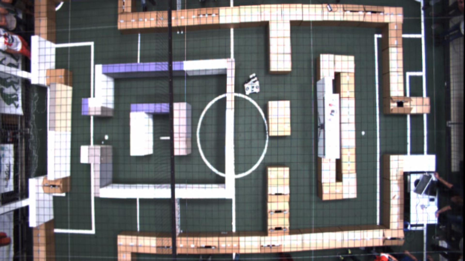
The software functions have multiple inputs and outputs and can be grouped by functionality. If data from the sensing component is used by a function from the skill component, the data is transferred between these components, this is referred to as an interface. A rough overview of the interfaces is shown in Figure 1. The dashed line represents that the actions of the robot will influence what the sensors measure.

Corridor Challenge
Repulsion & Angle correction


The first thing that was considered for the corridor challenge was some kind of repulsion from the walls to make sure PICO does not bump into anything. For the repulsion a simple version of an Artificial Potential Field is considered, which is given by the formula

where b is a scaling variable that can be used for finetuning, N1, N2, N3 and N4 mark the indexes of the laser data vector that determine which data is considered for the repulsion in a certain direction and \phi_i is the angle corresponding to measured distance distance r_i. Variable a is a correction factor for the width of PICO that can also be used during the finetuning.
For the calculation of the force in the forward direction, Fx, only laser data in front of PICO is used from index N2+1 to N3. All the other laser data is used for the calculation of Fy, the force in sideward direction. This is also shown in figure 2. The resulting netto forces are used as an input for the actuation function which is further explained below. Note that if the laser sees something at a very large distance or does not see anything at all, the returned distance is very small or even negative. Therefore all distances smaller than 0.01 meter are set to 10 meter.
For the angle correction all the laser data at the right side of PICO is considered. The smallest distance to the wall and the corresponding angle are found using a for-loop. After subtraction of 90 degrees, the resulting angle is used as input for the desired rotation speed. This approach can be interpreted as a torsional spring connected to PICO and is visualized in figure 3.
Actuation

The main functionality of the actuation script is to scale velocity signals that are sent to PICO in such a way that the constraints on maximum velocities are respected. Furthermore, effects of angle wrapping are compensated to create useful odometry data to rotate with a certain angle. Scaling of the translational speeds in x and y direction is done using

in which Fx and Fy are the force signals from the repulsion script sent to the actuation script. This is clarified in the figure on the right. If an angular velocity exceeds the maximum value, the angular velocity simply gets scaled back to the maximum angular velocity using
such that it makes sure that PICO will still turn in the right direction.
When using the actuation script to rotate with a certain angle, the script will in each iteration return a relative rotation angle. The script in which the actuation script is called then has to integrate this relative angle until the desired angle has been rotated. However, the angle from the odometry data can jump from –π to π of vice-versa. If this happens, the relative angle will not be correct and is adjusted by adding or subtracting 2π.
World model


Two types of nodes are detected by the scanNodes function and returned as a vector. The two types are:
- End nodes: These nodes are recognized using the SPIKE algorithm. When the difference between a previous data point and the next data point of the LRF data is above a certain threshold the node is stored.
- Corner nodes: The current data-point is a corner node if it passes the 90-degrees-test. This is a test that considers a previous data-point that lies at a set number of data points from the current data point, and a next data-point that also lies at a set number of points from the current data-point but to at the other side. Using the cosine rule, angles and distances to the three points, the length of the sides A and B as depicted in the Figure to the left, can be determined. Using the cosine rule, length C as shown in the Figure to the left, can also be calculated. Using Pythagoras, the length C can also be determined from A and B. However, this is only possible if the corner is 90 degrees. So, Pythagoras is applied and the calculated length of C is compared to the actual length of C. If the calculated length and the actual length are the same, then the corner is 90 degrees and thus a corner. Since these two values are never exactly the same and corners will never be exactly 90 degrees, margins are added to make the system more robust. Doing so creates a trade-off, more robustness means more chance of recognizing the corner, but it can also create the effect that not one data-point passes this test at a corner, but multiple data-points pass the test. For this reason a filter has been built that states that in a given range around a node, there can not be a second node.
The nodes are then used to in order to recognize the corridor and take the turn. The Node class (data type) is defined as follows:
- ID (int): The ID of the nodes are set from right to left (in the scanning direction of the LRF) starting at ID 0.
- Type (int): The types are defined in the header file of the world model library worldmodel.h. Two types are currently in use: Cornernodes and Endnodes.
- Location (location): For each node the Location class is used to track the position in both carthesian and radial coordinates relative to PICO. When the location class is updated using the radial coordinates the carthesian coordinates are updated automatically.
Making the turn
Driving between two walls can be easily done using the actuation, repulsion and angle correction code. To actually make a turn at the right moment to drive into the corridor, the corridor has to be recognized. From the world model, corner nodes and end nodes are received. We search for a corner node at the right and left of PICO (light purple area the figure below). If such a corner is found, and the distance to this corner node checked to see if the distance is reasonable (0.1m – 1.5m). Consider a corridor with the exit at the right, then the corner node will recognized at the right. The distance to the closest corner node present in the light green area in the figure below, is used to calculate the width of the corridor using the cosine rule. If no other corner node is recognized in the light green area or the recognized corner node is too far away, the distance to the first corner node (denoted with the number 2 in the figure below) is taken as half the corridor distance.
To take the corner, half of the corridor distance b is driven forward, during which the repulsion in forward direction is not used. After travelling b/2 meters, PICO stops and rotates 90 degrees. Then a distance of c+e is driven forward, where c is the distance as shown in the figure below, and e is a variable that can be used for tuning. This distance is driven forward to prevent PICO from recognizing corner node 2 again at his right and starts turning again before the corner is completely taken. For a corridor at the left, the exact same approach is used.

Result
In the end the corridor challenge was completed successfully. PICO seemed to miss the exit at first, but after some time the corner was recognized and PICO could take the turn. Because of the repulsion away from the wall, PICO moved towards the center of the corridor without bumping into the wall. In the end the corner node was not recognized because of a mistake in tuning. Nodes are recognized, but cannot overlap. A parameter governing the overlap radius was set to 0.5 meters. However by mistake a node was also set on PICOs' own position. This meant that when PICO approached the corner the node disappeared. When PICO moved sufficiently far past the corner the node was recognized again and the turn was made. Tuning the parameter to a 0.1 meter radius and testing again resulted in a direct and fast turn which could be executed in a robust manner.
The most important conclusion for us during the challenge was that we needed time to tune our parameters and remove small bugs from our code. This realization resulted in a discussion which drove our further design into a simpler direction in order to have enough time to robustly test the system.

Final design
Design decisions
To make a functioning robot, decisions have to be made with regard to maze solving algorithms. This chapter will focus on why and how the decisions are made. Three options were considered; the Pledge algorithm, Trémaux’s algorithm and the random mouse algorithm.
The Pledge algorithm lets the robot follow the wall either at its right-hand side or left-hand side (decided on forehand). Whilst following the wall, it counts the amount of corners taken. The counter is updated by adding 1 for a right turn and subtracting 1 for a left turn. If the robot is in its preferred direction (the counter is 0), the robot will not follow the wall. Instead, it continues driving straight forward until it sees a wall in front of it. It will then follow the newly encountered wall. The benefit of the Pledge algorithm is that the robot should always finish the maze in a finite time without keeping track of a world map. A downside is that this is not necessarily the fastest way to solve the maze. The robot may for instance drive past the finish just because it does not look at what is at its left side. Another downside is that it is quite sensitive for errors. The whole Pledge depends on the counter, if the counter gets mixed up, it may be possible that the robot will have to travel a lot of extra distance.
Trémaux’s algorithm, in contradiction to the Pledge algorithm, does require to keep track of a world map, which makes it a lot more complicated immediately. By marking the points that have already been visited, decisions can be made such that it is guaranteed to find the exit of the maze. This does not necessarily have to be faster than the Pledge algorithm. However, during the maze challenge, each group has two attempts. During the first attempt, Trémaux’s algorithm can be used to explore the maze and to find a way to the exit. In the second attempt, PICO can directly drive to the exit, because it already knows what path to follow, assuming that the first attempt was successful.
The final option we considered is the random mouse algorithm. This algorithm makes a random decision at each junction. Therefore the robot will eventually always find the exit of the maze, but this can take a lot of time.
Eventually, the decision has been made to use the Pledge algorithm. The main reason to do this is the fact that the complexity is limited, while it is still an efficient way to solve the maze. During the corridor challenge we experienced that it is very important to tune the configuration parameters on the actual robot instead of the simulator. Therefore the decision has been made to create a robust realization of a relatively simple algorithm (Pledge) instead of a complex algorithm (Trémaux). In other words, our focus is on finishing the maze challenge rather than implementing the most complex algorithm. Right after the corridor challenge the world model could not yet detect walls, only nodes. Together with a possible redefinition of nodes we thought it would be wise to choose Pledge in order to avoid making a map, which would be finished at the last second or not at all. Therefore the world model team focused on recognizing doors, while the path finding teams focused on implementing Pledge.
After choosing the Pledge algorithm, a decision had to be made on how to take turns. We considered two options:
1. Rotate while standing still
2. Keep driving while rotating
Both methods have their advantages and disadvantages. The advantage of the first one is its simplicity. We can just create a state for taking corners in which PICO drives forward, rotates 90 degrees using odometry data and drives forward again. Each time when we call the state, we can update the Pledge counter. When using the second approach, it is less straightforward to detect when the corner has been taken. Regarding the robustness of the Pledge counter, this might form a problem. However, for PICO to find the exit as fast as possible, it is not favorable to stand still while cornering. In that sense, option 2 would be better. We decided to try both methods and choose the one that works best in practice. In the end, option 1 resulted in the most robust Pledge counter, which is needed for solving the maze. Therefore we continued with that strategy.
Another important design decision is about the use of a world map. Although this is not necessary when using the pledge algorithm, it can still be beneficial. Basically, all we need to do is follow the wall on PICO’s right if the pledge counter is unequal to zero. This can be done using a space recognition algorithm, which will be discussed later. On the other hand, using a world model, we can implement feature detection to recognize junctions and base our decisions on that. However, during the corridor challenge we experienced that a small error in detecting corners can already have a large impact on the behavior of PICO. You completely base the decisions on corner nodes that appear on certain locations, which is risky if the robustness of these nodes is not fully reliable yet. The design decision has been made to only use a world map for door detection. Driving using the pledge algorithm will be done with the space recognition algorithm. In this manner, we aim at a robust way to solve the maze.
Interface

After the corridor challenge, the software architecture was changed a bit. The software still consists of five main parts: actuation, skill, sensing, worldmodel and taskmanager. These different software parts with their corresponding in- and outputs are depicted in the figure to the right. The software architecture is globally explained in this section. The important parts are further explained in the following sections.
Taskmanager
The taskmanager is the top part, which controls the whole software. Data comes in via the skill and sensing part, and data is sent to the strategy and actuation part. Based on the data from the other parts, the task manager makes decisions on what to do. First, it calls the variable ‘door detected’ to check whether PICO is in a door area. Then it will go to the initial state ‘start’ in which the startup procedure is implemented. It checks if there is a wall on the right side of PICO, and PICO will be aligned to this wall. When PICO is aligned to this wall, it will go to the following state ‘straight_pref’. In this state, PICO drives in its preferred direction and calls the boolean vector from the space recognition skill. This information is sent to the strategy skill, which sends the direction and state back. Based on this information it will stay in the case ‘straight_pref’ or switch to the state ‘straight’, ‘turn_left’, ‘turn_right’ or ‘turn_180’. When it stays in the same case, it will call the force struct from the repulsion skill. After that, the actuation vector is sent to the actuation part. When it switches to a state ‘straight’, the same is implemented as in the state ‘straight_pref’, but now the distance to the wall is added. This is implemented as a virtual spring, which will be further explained in the Maze solving algorithm section. In the states ‘turn_left’ and ‘turn_right’, the odometry data is used to check whether PICO has rotated enough.
Actuation
The input of the actuation part is an actuation vector, which contains the horizontal, vertical and angular velocity or a door request. The actuation part consists of four sub parts: move, stop, rotate and opendoor. The taskmanager decides which part is called. In the actuation part, the velocity is scaled, such that it does not exceed the maximum velocity. When the normalized velocity is calculated, this is sent to the actuators. When opendoor is called, an ‘opendoorrequest’ is sent to the actuator such that it will ring a bell.
Sensing
In the sensing part, the odometry and LRF data are obtained. The LRF data is directly used in several functions. For the odometry data, the difference between the previous and the current odometry data is calculated, this way the angle is unwrapped and the relative rotation can be calculated.
World Model
The world model is a function that detects nodes using the LRF data. Using various algorithms, the data from the LRF can be filtered and the most important data points are saved as nodes. Important nodes concern mostly nodes that lie on the end of walls or that are corners. Using these nodes, the current world that PICO sees can be made. These nodes are used to recognize doors.
Skill
The skill part contains the skills of PICO, which are the calculation of the repulsion, the space recognition, the door recognition and the strategy. In the repulsion part, the repulsion forces are calculated using the LRF data. In the space recognition part, it is checked whether there is space to the left, right or front using the LRF data. In the door recognition, the door areas are calculated using the nodes from the World Model. When PICO is in a door area the Boolean 'door detected' will be true. The strategy part gets the boolean vector of the spaces from the task manager. Based on this spaces boolean vector, the strategy part will update the direction and desired state based on the Pledge algorithm.
Visualization
The visualization is not a functional part of PICO, but it is used to visualize what happens in real time. The input is a vector with nodes, which are transformed to dots, lines and numbers in the visualization. It is mainly used to check if the "node detection" and "door recognition" are working correctly.
Space recognition

This function determines whether there is space or an obstacle to the left, right and top of PICO. In the config file, the beam width is determined in degrees. This value is converted to radians and used to determine which LRF data points should be checked. As can be seen in the figure, there are 3 beams to be measured: left of PICO, above and to the right of PICO. By default, all spaces are defined true. If one measured LRF point is below the threshold value, indicated with an orange circle, the space_x variable will be set false. The threshold for the forward distance can be tuned independently of the others. The forward distance is slightly smaller than the other distances. This means that PICO will detect an obstacle in front of him later and will react later to this. This way a better wallfollowing can be realized. The function needs the scan information from the LRF as an input and will output the variables space_left, space_top and space_right.
Code
This relatively simple functionality is neatly implemented as can be seen in this code snippet. The code is simple, understandable, has a clear purpose and can be tuned fully from the config file.
Maze solving algorithm
The Pledge algorithm is chosen to solve te maze. The pledge algorithm has a preferred direction and counts the corners the robot takes. A left turn counts as -1 and a right turn as +1. When the counter is 0, the robot goes in its preferred direction. The pledge algorithm is implemented in the following manner:
- If PICO is driving in preferred direction:
- if space_top = true: Go straight in preferred direction
- if space_top = false & space_left = true: rotate 90 degrees left
- if space top = false & space_left = false & space_right = false: rotate 180 degrees left
- Else
- if space_right = true: rotate 90 degrees right
- if space right = false & space top = true: go straight
- if space_right = false & space_top = false & space_left = true: rotate 90 degrees left
- if space_right = false & space_top = false & space_left = false: rotate 180 degrees left
In Figure 3 PICO is depicted with three beams: space_left, space_right and space_top. All beams are using only 5 degrees of LRF-data.

Code
The Pledge algorithm is implemented as a function that needs the current counter and all the spaces. It will output the updated counter and the desired state to be in. Since the interpretation of the spaces is straightforward, the Pledge algorithm can be implemented in a straightforward manner. By thinking out the algorithm first, the right hand follower was implemented with no problems at all. The function also gives feedback to the programmer in which state PICO currently is. This Pledge function is another piece of code that represents our neat and straightforward manner of coding, with which we made a very robust maze solver.
Repulsion & wall following
How the repulsion and angle correction are working is already explained in the section Corridor challenge. The final repulsion and angle correction are not changed very much in the final design, only some values are tuned. The wall follower is added in the final design, which makes sure PICO stays at a desired distance from the wall. The wall follower is implemented as a virtual spring. When PICO is too close to the wall, the repulsion becomes very high and PICO will be pushed from the wall. When PICO is too far from the wall, the virtual spring will give a force. Therefore, PICO will be pulled to the wall. Between the repulsion and virtual spring is some threshold, such that the forces are zero in that area. This makes sure that PICO does not correct itself the whole time.
Taking turns
Turning right
Taking a turn isn't so easy as it sounds. When following a wall PICO stays nicely aligned and close to it. When PICO detects space it wants to turn right to follow the wall (assuming the Pledge counter is not 0). However, if PICO turns too soon he would be very close to the corner. This would result in repulsion helping PICO to stay away from the corner, but not in a nicely made turn. Therefore PICO drives a small distance forward before rotating 90 degrees. After that the robot indeed makes the turn of 90 degrees. It does a 90 degree turn by measuring odometry data. After PICO is rotated, we do not want to measure immediately after that, for that would result in an open space to the right of PICO and it will again rotate to the right. Therefore PICO first looks for an obstacle to his right, seeing an obstacle here means that he indeed is far enough that he indeed made the turn. Now PICO can remain following the wall. The desired state is set to 'straight' again.

Deadlock prevention
It could happen that PICO thinks there is space to his right, while it is actually not. PICO could either be too far away from the wall, or it could be very close to a wall which has a small gap. In both scenarios a faulty space_right would be detected, making PICO turn right. What will happen is that PICO will turn right and search for an object to his right. After the turn, PICO is facing the wall in front of him and he wants to go forward. However, repulsion will keep PICO from bumping into the wall. To avoid a deadlock situation, a counter keeps track of the time. After 10 seconds of trying to find an obstacle to the right of PICO, it will take a left turn again in order to follow the wall again. This indeed prevents deadlock, it was even shown in the maze competition in the fast configuration.

Turning left & 180 degrees
Unlike turning right, turning left is fairly easy. When PICO detects an obstacle to the right and in front of him, the only option is to go left. After turning left 90 degrees, PICO can immediately start following the wall again. When turning 180 degrees it is exactly the same case, except that PICO will turn 180 degrees immediately.
World model
In order to recognize door areas a world model is constructed which uses landmark detection. Landmarks are defined as nodes, which are points in the LRF-data with certain properties which are collectively defined as either "end" nodes or "corner" nodes. The world model library provides a function which can be used to detect nodes in the landscape.
    /*!
      \brief scanNodes  Scan for nodes and return a vector of the detected nodes.
      \param scan       A scan of the environment containing angle and distance data of the LRF.
      \return Vector containing nodes detected during the scan.
    */
    std::vector<Node> scanNodes(emc::LaserData scan);
The resulting node vector in this case is then used to recognize door areas using the doorCheck function, which returns true when a door area is detected and PICO is located there.
Node class
The Node class (data type) is defined as follows:

- ID (int): The ID of the nodes are set from right to left (in the scanning direction of the LRF) starting at ID 0.
- Type (int): The types are defined in the header file of the world model library worldmodel.h. Two types are currently in use: Cornernodes and Endnodes.
- Location (location): For each node the Location class is used to track the position in both carthesian and radial coordinates relative to PICO. When the location class is updated using the radial coordinates the carthesian coordinates are updated automatically. The axis are defined the same way as during the corridor challenge.
- Connections (std::vector<int>): A vector of node IDs. For each connected node the ID is stored in this vector. Thus it is possible to determine which nodes are connected by walls and which are not.
- LRFindex (int): Index in the LRF scan of the particular data point corresponding to the current node. It is mainly used to determine the connection vector.
Node recognition

The world model is based on two types of nodes: endnodes and cornernodes. Finding nodes is done with the following checks over all data-points:
- The current data-point is a cornernode if the distance between the current data-point and the next data-point is larger than a given value and that point lies closer than the one it is compared with. This type of corner is basically has a 270 degrees corner. As an example, a T-junction consists of two of these type of corners. The closest point has to be the cornernode since it blocks the view of further vision. The next node is further away and one point on its side can not be seen because the corner is in the way.
- The current data-point is a cornernode if is passes the 90-degrees-test. This is a test that considers a previous data-point that lies at a set distance from the current data-point, and a next data-point that also lies at a set distance from the current data-point. Using the cosine rule, angles and distances to the three points, the actual distance between the previous data-point and next data-point can be determined. Using the cosine rule, the distance between the next data-point and current data-point, and previous data-point and current data-point can be determined. Having two sides, the third one can be determined using Pythagoras. However, this is only applicable when a corner is 90 degrees. Therefor the result of this calculation can be compared with the actual value, which was determined using Pythagoras. If these two values are the same (or have a certain margin), then the corner is 90 degrees. The recognition was modified slightly to set the previous and next data point based on distance, and not on a number of data-points as was done during the corridor challenge. The result is a more intuitive parameter to tune the corner node recognition.
- The first check, was a way to determine a cornernode. The closest data-point was then considered the cornernode, since it blocks the view. The point that lies next to it and is further away, is also called an endnode. This was chosen because this node lies at the end of the visible world of PICO at that particular moment.
- A data-point that lies at the maximum range or at the maximum angles is considered an endnode.
The visualization of the corner nodes and the end nodes serves to debug and tune the object recognition.
Several tunable parameters are associated with the node recognition, which mostly deal with margins associated to the ways nodes are recognized. For example, a tunable parameter exists for the minimum distance two nodes need to be apart in order for the data point to be considered an endnode. A complete list with description is also available in worldmodel.h.
Wall recognition
In order to recognize whether nodes are connected the LRF index of the subsequent nodes is checked in order to see whether nodes are set at subsequent indexes of the LRF data. Two nodes can only have subsequent LRF indexes when the are separated by a large distance because of both the SPIKE check which compares distances, and a tunable parameter which determines the allowed overlap of nodes. Thus the nodes are not connected when the check is true.
Each node is checked in sequence. A connection is thus always added "backwards", connecting the node checked to the previous one by modifying the Connections variable of both.
Door recognition
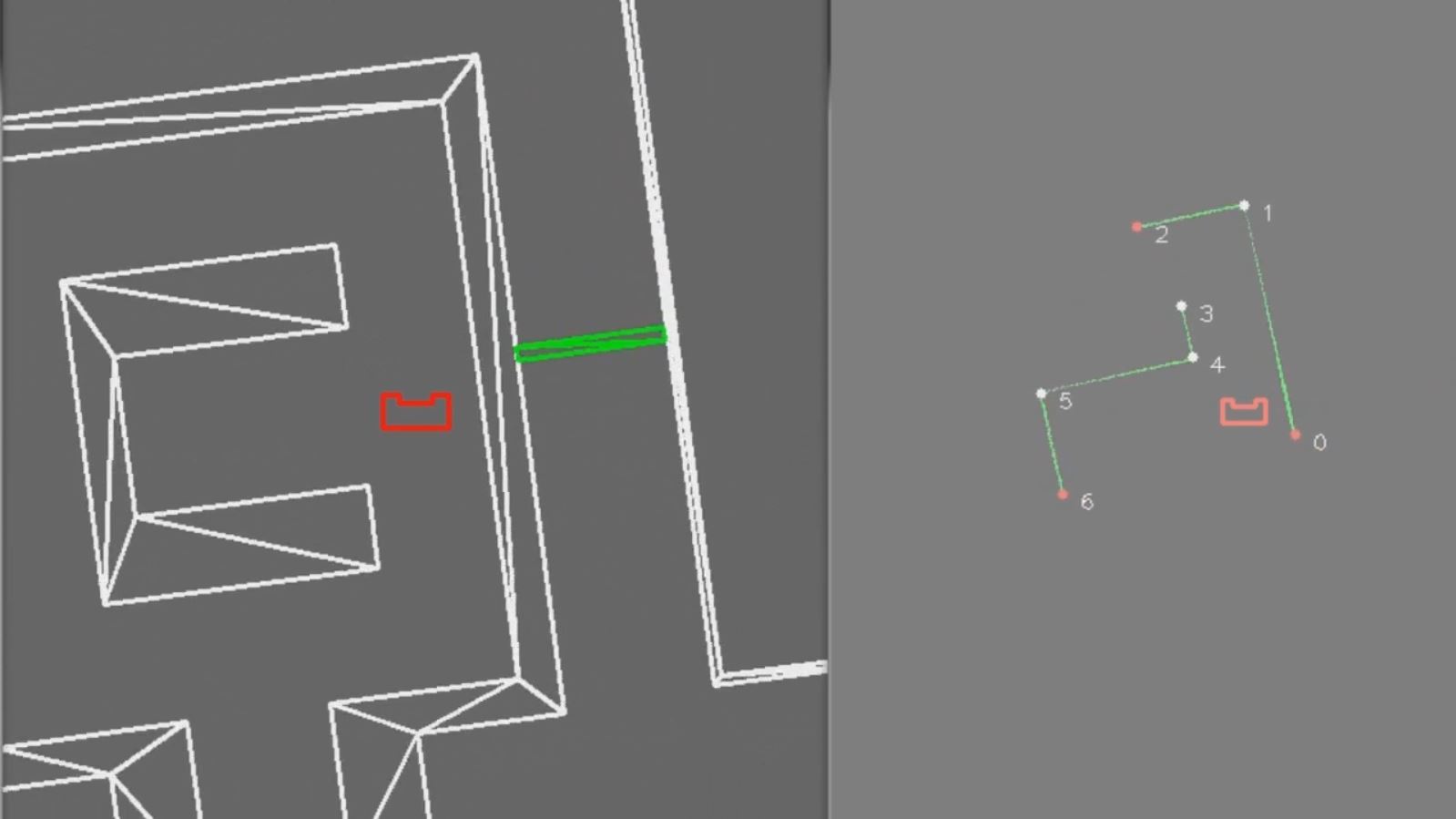
The doors are recognized based on the end- and cornernodes. It is known in advance that the node numbers are ordered depending on the angle of the LRF. The first node lies at the lowest recognizable angle, the last node at the highest recognizable angle. Based on this we can do several checks to see if a door should be recognized. The door check is done with a for-loop over the first to the fourth last nodes. This is because four nodes are required to check if it is a door. Let’s consider a certain node that needs to be checked, then the three following nodes are also considered to determine whether these four nodes make a door.
The first check, is a simple check that checks the absolute distances between the four nodes. Let’s consider four nodes that lie after eachother. The distance between the first two nodes has to be at least 0.3 meter according to the given requirements. Then the distance between the second and third node has to be at least 0.5 meter, but can at a maximum be 1.5 meter. The distance between the third and fourth node should once again be at least 0.3 meter. On each of these distances, margins are added to increase robustness. If a node passes this test, then it proceeds to the second check. If it does not pass this test, then it can’t be a door by definition and thus it not necessary to do the other tests.
The second check determines if the first and fourth node are on the same side of the line through node 2 and node 3. This is to check if it is actually a corridor and not a S-curve. An example of this is shown in the figure below. The left ‘door’ would pass this test whilst the right one would not. To check if the nodes 1 and 4 lie on the same side, the following equation is used:

In this equation are x and y are the relative coordinates with respect to the robot of the points that do not lie on the direct edge of the door (in the figure above these are nodes 1 and 4). x1, y1, x2 and y2 are the coordinates of the nodes that lie on the sides of the doors (thus node 2 and 3 in the figure above). This means that variable D needs to be computed twice, once for node 1 and once for node 4. If the sign of these two variables becomes the same, then these points lie on the same side of the door and the following check can be done.
The third check makes sure that the nodes are of the correct type. As stated before, we have two node types; endnodes and cornernodes. Nodes two and three should by definition be cornersnodes. If the two nodes are both cornersnodes then these two nodes are connected and thus it could be a door. The other two nodes can either be endnodes or cornernodes.
The fourth check calculates the angles of the two cornernodes. This needs to be done to make sure that the third and fourth, and first and second node are connected. This check is simply done using the same algorithm that was used for corner detection.
The fifth and last check, creates a door area based on the location of the door. The robot needs to be within this door area before it may ring the bell. Officially this should be a separate check since it does not belong to checking whether it is a door or not. However, it would not be useful to check whether a door is recognized, but not to check if the robot is within the door area. For this reason and the reason of simplicity, this check is done within the door recognition.
Code
The code of the Worldmodel can be found here. It takes care of a complex task, namely recognizing nodes and door areas, by dividing the code into clear cut function that can be called to determine whether nodes are present in the LRF data. It is nicely structured and executes complex tasks and new checks can easily be added and deleted to suit new insights.
Maze challenge
An epic video of our maze challenge can be found on Youtube. In this attempt, everything was executed flawlessly by PICO. Our code was robust enough to solve the maze, and it was even the fastest time (2:34) of all groups that completed the maze.
The maze has also been solved in simulation, the safe version completed the maze in 2:17 and the fast version in 1:36.
The safe version was our main focus and the fast version was therefore not tested extensively. This resulted in an error in the Pledge counter during the maze challenge. PICO was still able to complete the maze, but because of the error it would be slower than the safe version.
The a-maze-ing attempt made us the proud winners of the maze challenge!

PICO, you will be missed.
Code we're proud of
These codes are already mentioned at the relevant chapters, but here's a recap of the codes we are proud of.
The detect spaces functionality is neatly implemented as can be seen in this code snippet. The code is simple, understandable, has a clear purpose and can be tuned fully from the config file.
The Pledge algorithm is implemented as a function that needs the current counter and all the spaces. It will output the updated counter and the desired state to be in. Since the interpretation of the spaces is straightforward, the Pledge algorithm can be implemented in a straightforward manner. By thinking out the algorithm first, the right hand follower was implemented with no problems at all. The function also gives feedback to the programmer in which state PICO currently is. This Pledge function is another piece of code that represents our neat and straightforward manner of coding, with which we made a very robust maze solver.
The code of the Worldmodel can be found here. It takes care of a complex task, namely recognizing nodes and door areas, by dividing the code into clear cut function that can be called to determine whether nodes are present in the LRF data. It is nicely structured and executes complex tasks and new checks can easily be added and deleted to suit new insights.
Conclusion and recommendation
As mentioned before, the maze challenge was won by our group. We focussed on implementing a simple system that we could test and tune over a complex implementation, which turned out to be a success.
Looking back on the project, it can be concluded that most decisions were well chosen. Deciding that the wall-following algorithm and Pledge should not depend on the world model was a good way to split up the work without making groups dependent on each other. Because of this, small groups of two people could work together and were responsible for a certain part of the code. Making the two parts not dependent on each other has the benefit that the two parts could be developed completely independent of each other. The downside is that the world model has a less important role in solving the maze. Making the algorithm dependent on the world model could make the whole more robust, since the world model only uses select data to reconstruct the maze. For instance, a small gap between two walls could now have given quite a problem. If the wall-follower would depend on the world model, then two nodes were simple connected which would then be seen as a wall. If there would be a small gap, the robot would ignore this completely. Note that with the current world model, this extension can easily be made. However, if the world model does not function very well and for example mis places a corner node, you have a big problem. We experienced this during the corridor challenge, where a small bug in the world model code resulted in driving past the corridor. Fortunately, PICO still found the corridor due to the fact that the repulsion pushed him toward the gap in the wall.
The Pledge algorithm itself worked as desired, but it is of course not the fastest way to solve a maze. The simplicity of this algorithm however makes it very suitable for this project due to the time available. If more time was available after the maze challenge, then more difficult algorithms such as Trémaux could be considered.
There are really not many things that we would change if we could start over. We strongly recommend to make appointments on when to work on the project. For instance, our group worked on Monday two hours together, as well as four hours on Friday. Programming together gives the option to discuss things quickly when a problem arises, to help each other when there is a problem and most importantly; to communicate about how parts of the code work and what they should output.
The Pledge algorithm was the best choice for the given time, a more complex algorithm would probably have decreased the robustness and more errors could have occurred during the maze challenge. In the beginning of the project it seems like there is quite some time available, but the last week is almost completely spent on bringing the various parts together and on tuning PICO to its best performing configuration.
Another decision that was well made, was not to focus on the corridor challenge too much, but mainly on the maze challenge. The corridor challenge was simply a check in the middle of the project to see how well our code worked so far. Unfortunately we didn’t win the corridor challenge, but the world model was already way more advanced then needed by the time the corridor challenge was done. This was because the world model was created for the maze challenge and not directly for the corridor challenge. The corridor challenge was also a good test to think about how to take a corner, which is harder than it seems at the start of the project.
Doing this project was a great introduction into the world of creating software. Besides learning how to program in C++, work in Qt creator and working with Linux, it was especially interesting to see that the initial software design/architecture is very important during the rest of the project. If this architecture is not well thought about, this will lead to problems halfway the project. It should be clear which part does what. Also it should be clear which parts depend on each other and that agreements are reached on the interfaces between the different components of the software.