Embedded Motion Control 2015 Group 4

Authors: T. Cornelissen, T van Bommel, M. Oligschläger, B. Hendrikx, P. Rooijakkers, T. Albers

Requirements and function specifications

Problem statement

The software design process starts with a statement of the problem. Although all the details of the assignment are not yet knwon at this point, we can best summarize the statement with the following sentence:

Design the software in C/C++ for the (existing) Pico/Jazz robot that enables to find the exit of an unknown and dynamically changing maze in minimal time.

Requirements

A (draft) list of the requirements contains the following points:

• Exiting the maze in minimal time.
• Avoiding damage of the robot and the environment.
• Robustness of pathfinding algorithm with respect to maze layout.
• Design software using modular approach.
• Implement algorithm using only available hardware and software API's.
• Manage code development with multiple developers.

Existing hardware interfaces

• The Pico/Jazz robot with customized inner workings and a robot operating system with C++ API's.
• A (still unknown) wheelbase layout of which the possible DoF/turning radius is a design constraint.
• A lasersensor and acoustic sensor of which the range-of-visibility is a design constraint.

Unknown design constraints

• Simulation environment for code testing?
• Location of sensors and wheels relative to robot fixed frame?
• What data can we extract form the sensors?
• What does the maze look like? How do the doors operate?

Main focus point in the first two weeks

• Learn basics of C/C++ and software development.
• Determine the layout of the robot and the possibilities of the sensors and wheel structure.
• Become familiar with the integrated development environment.
• Explore the possibilities of th API's (how much postprocessing of the aquired sensor data is necessary and what techniques must be learned?).

Software design strategy

The figure below shows the overview of a posible software layout. The skill functions can be assigned to different programmers that are also responsible for exploring the API's and gathering details about the hardware. The maze solving strategy can be handled separately and the supervisory controller is the brain of the robot combining all the information. File:Maze example.pdf

Composition pattern

The task of the robot is to solve a maze autonomously. In order to do this a piece of intelligent software has to be developed. The software must be able to give on the base of stimuli and knowledge valid instructions to the hardware. In order to obtain a reliable system behavior it is wise to use a structured system architecture. Our solution for solving a maze can be seen as constructing a subsystem that is connected to other systems. An approach of defining our system is by divide the system in structure, behavior and action in an appropriate way. Herein the structure describes the interaction between behaviors and activities; this is the composition or the system architecture. The behavior is the reaction to stimuli, a possible model for this is the Task-Skill-Motion model. The activity is responsible for how the behavior is realized (the execution of code).

In the scheme below the Task-Skill-Motion model of our solution is shown, this model has functioned as a base for our design.

Task-Skill-Motion model

• The User Interface Context provides the communication with the user, this is a bilateral exchange of instructions/information between user and software/robot.
• The Task Context functions in our case as a kind of supervisor. It feeds and monitors the separate skills.
• In our Skill context a distinction is made between skills that are dedicated to: solving the maze, motion skills and service skills.
  • The Maze solving skills produce optimal decisions for solving the maze, it also translates and maintains the data in the semantic world model.
  • The motion skills produce instructions for the hardware, it moves the robot in corridors and corners and open spaces.
  • The so called service skills deliver a service to the other skills. For example the laser vision skills are responsible for detecting junctions, calculating alignment errors and producing a current state local mini map of the world. For global localization and mapping of the global world a SLAM implementation is used.
• The environmental context contains a model of the world. This model can be provided by the user or build, expand and maintained by the skills. The semantic model for solving the maze contains nodes with additional information at junctions in the form of a graph. On the other hand we have a 2d model of the world in the form of a list of lines and corners used for the global localization (this is for localization also very semantic).
• The Robot Abstraction performs the communication between our software and the hardware. This shell is in our case provided, however we added a very thin layer on top (between our software and the Robot Hardware Abstraction). This layer passes the parameters that have to do with the difference between the dynamics in the real robot and the kinematic model in the simulation (this mainly about motion control gains).

Implementation of software

Our software design is based on a principle that is also used in a programmable logic control (plc). The software does not run on an industrial plc but on the embedded Linux pc in the robot. Our program consist of a main loop that is executed with a frequency of 10Hz. Within the loop the following process sequence is as much as possible followed:

• Communicate
• Coordinate
• Configure
• Schedule-acts
• Act
• Communicate
• Schedule-prepares
• Tasks’ prepare
• Coordinate
• Communicate
• Log

such that the whole process can be executed in serial.

Pseudo code of our main loop

In the figure above a pseudo code of our approach is shown. The advantages of this setup are:

• No multithreading overhead
• Maintainability
• Predictable behavior

On the other hand the disadvantages are:

• No prioritizing
• Calculations made every loop
• No configurability

Actual code

The code snippet below contains the code used in the actual maze challenge. Code snippet: https://gist.github.com/anonymous/5bdc865a5d10a7a7c312

Laser vision

Compass function

This function measures the angular misalignment of the robot with it's environment. The compass function gives a valid estimate of the angular misalignment under the following assumptions.

Assumptions:

• The world consists of mainly straight lines.
• All the lines cross each-other approximately with an angle which is a multiple of the world angle (when for example all the angles are perpendicular then the is 90 degrees)
• The current misalignment of the robot with it's environment is small: [math]\displaystyle{ \theta_{robot}\lt \lt 0.5\cdot\theta_{world\,angle} }[/math]. This implies that the compass function is unreliable during large rotations.
• There are enough sample points (preferably in front of the robot) to ensure that lines can be detected in the so called trust area.
• The trust area is defined as a bounded square around the robot which is aligned with the robot frame. Only the samples in this square are used for the compass function calculations. As is shown in the figure below.

Compass function

Reference line

Approach:

We are searching for a reference line from which we can calculate the angular misalignment of the robot. This calculation proceeds in the following sequence: First the laser data is expressed in a orthogonal frame (fixed to the robot). A line through point [math]\displaystyle{ [x_i,y_i] }[/math] can be described in polar coordinates as [math]\displaystyle{ p(\alpha)=x_i \cos(\alpha)+y_i \sin(\alpha) }[/math] where [math]\displaystyle{ p }[/math] and [math]\displaystyle{ \alpha }[/math] are unknown parameters. We want to find a [math]\displaystyle{ \alpha\in[0,\pi] }[/math] and a [math]\displaystyle{ p\in [-p_{max},p_{max}] }[/math] where [math]\displaystyle{ p_{max}=\sqrt{(2\cdot trust\,area\,size)^2} }[/math] is half the trust area diagonal. The Hough transform [1] gives a procedure to find [math]\displaystyle{ p }[/math] and [math]\displaystyle{ \alpha }[/math]. The procedure is as follows: for each [math]\displaystyle{ [x_i,y_i] }[/math] in the trust area and [math]\displaystyle{ \alpha\in[0,\pi] }[/math] the value of [math]\displaystyle{ p(\alpha) }[/math] is calculated.

The calculated [math]\displaystyle{ p }[/math] values are round to the closest value in a discrete set. The Hough parameter space can in this case be interpreted as a 2 dimensional grid where the first axis represents the value of [math]\displaystyle{ \alpha }[/math] and the second axis the [math]\displaystyle{ p }[/math] value, where for each solution of [math]\displaystyle{ p }[/math] a value of one is added to the corresponding cell in the grid. The parameters of our reference line are the parameters that corresponds to the highest value in the Hough parameter grid.

The Hough transformation is shown in the following figure. The x and y values of the laser measurements are shown on the left. On the right the Hough space is shown, where the red line represents the current [math]\displaystyle{ \alpha }[/math] value of our reference line.

Only the [math]\displaystyle{ \alpha }[/math] parameter is in this case of interest. Since we assumed that the angular error of the robot with its environment is small we calculate the misalignment as the smallest difference between the parameter [math]\displaystyle{ \alpha }[/math] and a multiple of the world angle (in other words it does not matter for the result when we find a reference line parallel to the robot y axis instead of a line parallel to the y axis).

Applications:

The result of the compass function can be directly used to reduce the angular misalignment of the robot with its environment. This is accomplished in the form of a simple gain feedback control rule: [math]\displaystyle{ \omega_z=K_ze_z }[/math] where [math]\displaystyle{ \omega_z }[/math] is the rotation velocity, [math]\displaystyle{ K_z }[/math] is a control gain and [math]\displaystyle{ e_z }[/math] is the angular misalignment found by this function. The other application of the compass function is to align the mini map with the robot’s environment.

Minimap

This function creates from the sample data a small map around the robot. The map indicates areas where obstacles are and where not. The purpose of the mini map is to make it possible for sub functions to simply and flexibly detect maze futures such as side paths, maze exits and position errors it forms also an important input for the world model.

The following points are of interest in this function:

Assumed in the compass function was that the angular misalignment is small and will converge to zero since it will be compensated by a controller. Therefore we align the mini map not with the robot frame but with the world. A second trust area is created, which forms the bounds of the mini map (with different dimensions as in the compass function). The map is discretized in blocks of a specified size (x-y accuracy in [m]).

In the figure above is shown:

• In A. the laser range finder data is transformed to a orthogonal frame:[math]\displaystyle{ x_i=r_i\cos(\theta_i) }[/math] and [math]\displaystyle{ y_i=r_i\sin(\theta_i) }[/math]
  where [math]\displaystyle{ \theta_i=\theta_{increment}i+\theta_{min}-e_z }[/math].
• In B each sample i is fit in a block and when there is a sample in the block then the block/pixel value is changed to 1. The remaining blocks are left 0.
• In C a collision detection is applied to detect areas where there are no obstacles. This is a simple line search for each angle from the middle (robot position) up to a block or the trust area border. This is done for all the angles in the range of laser range finder. The maximum allowed angular step is the angle that a rib of a block on the thrust area border makes.
• In D the final binary mini map is shown (the center cell represents the robot position).

In the figure below is shown that the minimap is aligned with the world rather than with the robot, this simplifies the calculations in the feature detection functions. A simple gain feedback is used to align the robot with the world.

Junction detection

Junctions can be detected by applying a simple analysis of the Minimap. The basic principle that we are using is to try to fit a box of an appropriate size in the side-paths. If the box fits in the side-path then also the robot fits in the side-path. We detect side-paths on the right, on the left and in front. In addition we check if the side-paths are probably doors by scanning the depth of the junction. If there are no side-paths detected a distinction between corridor or dead end is made. Approach:

• The analysis starts with measuring the size of the corridor [math]\displaystyle{ a_1 }[/math] and [math]\displaystyle{ a_2 }[/math] in the figure below.
• Then is measured if the robot is in the begin of a junction by checking if there is a sharp change in corridor size just in front of the robot on one of the two sides (measurement [math]\displaystyle{ a_3 }[/math] or [math]\displaystyle{ a_5 }[/math])
• The next check is if the green box fits in the side paths, which is the case when [math]\displaystyle{ a_4 }[/math] and [math]\displaystyle{ a_6 }[/math] are larger than the box size (current box size is 20x35 cm).
• Then the largest bound [math]\displaystyle{ a_4 }[/math] or [math]\displaystyle{ a_6 }[/math] is taken to build up the analysis for the path in front.
• Again when [math]\displaystyle{ a_7 }[/math] and [math]\displaystyle{ a_8 }[/math] are large enough such that the box fits in it, then a path in front of the robot is also detected.

First step in junction detection

• The door detection is an additional test on the junction detection, a possible door is defined as a junction with a limited depth. If an already detected junction has a limited depth then it can be a door. The process is approximately the same as in the junction detection and is indicated with the blue measurements [math]\displaystyle{ b_{1,2,3,4,5,6} }[/math] in the image below.

Detect possible doors by checking the depth of a junction

• The final output of this function is the type of corner and the dimensions [math]\displaystyle{ d_{1,2,3,4} }[/math] indicated in orange in the figure below. With these dimensions a path can be constructed through the corner.

Output parameters of the junction detection function

• A dead end is detected by detecting a limited free area in front of the robot.
• An open area is detected by large free area on the left, right or completely free area in front of the robot.

Y position error (center error in corridor)

The Y position error is the distance of the robot to the middle of the corridor. The approach is to calculate a left and a right bound in front of the robot (we don’t look sideward but in front of the robot). From these bounds the following center error is calculated:
[math]\displaystyle{ e_y=\frac{k_{left}+k_{right}}{2} }[/math]
This center error is used to control the robot to the middle of the corridor with control rule: [math]\displaystyle{ v_y=K_ye_y }[/math]

Bounds for calculating the y-error (corridor challenge)

Improved y-error (limited view of depth)

In the figure below an example is shown of the correction of the robot alignment with only a simple gain feedback in y-direction. Observed can be that the robot already aligns before it enters the corridor.

Side path detection (as was used in the corridor challenge)

This function triggers when there is a side path found. The function calculates a front and a back bound. During the corridor challenge this function triggered the rotation function (which was tuned way to slow) under the conditions:

[math]\displaystyle{ |k_{front}|+|k_{back}|\gt minimal\,door\,size }[/math]

and

[math]\displaystyle{ |k_{back}|\gt |k_{front}| }[/math]

Bounds for side path detection (during corridor challenge)

Exit detection (as was used in the corridor challenge)

If there is nothing in front of the robot then it is an exit.

Exit detection (during corridor challenge)

Laser vision in action

In the figure below a simulation of a corridor challenge is shown, it illustrates the robustness and simplicity of object detection in action. On the left the simulation of the robot trough the corridor is shown and on the right the mini map is shown.

World Model

Extended Kalman Filter

The Kalman Filter can be used in the SLAM algorithm to predict the location of the Pico in the maze and predict the location of the landmarks.

The position of the Pico can can be described by an x and y position with angle because of orientation. Both the odometry and laser data can be used to measure the Pico's positon. Especially the odometry has significant measurment noise. The figure below shows the position parameters for the Pico.

Here the x, y and [math]\displaystyle{ \alpha }[/math] are the position states. And [math]\displaystyle{ V_{x} }[/math], [math]\displaystyle{ V_{y} }[/math] and [math]\displaystyle{ \omega }[/math] are control inputs to the base. So the control and state vector becomes:

[math]\displaystyle{ x_{k} = \begin{bmatrix} x_{pos,k}\\ y_{pos,k}\\ \alpha_{k} \end{bmatrix}, u = \begin{bmatrix} V_{x}\\ V_{y}\\ \omega \end{bmatrix}, (\omega = \dot{\alpha}) }[/math]

To update the position state based on a motion model of the Pico the following equations are used: [math]\displaystyle{ x_{k+1}=f(x_{k},u_{k})= \begin{bmatrix} x_{k} + \Delta t(V_{x}cos(\alpha_{k}) - V_{y}sin(\alpha_{k})) \\ y_{k} + \Delta t(V_{x}sin(\alpha_{k}) - V_{y}cos(\alpha_{k})) \\ \alpha_{k} + \omega\Delta t \end{bmatrix} }[/math]

These equations are non-linear and that is the main reason why it is necessary to use the Extended Kalman Filter. The Jacobian used to update the covariance is the derivative of the above model:

[math]\displaystyle{ J = \frac{\partial f }{\partial x} = \begin{bmatrix} 1 & 0 & -\Delta t(V_{y}cos(\alpha_{k}) + V_{x}sin(\alpha_{k}))\\ 0 & 1 & \Delta t(V_{x}cos(\alpha_{k}) - V_{y}sin(\alpha_{k})\\ 0 & 0 & 1 \end{bmatrix} }[/math]

At first a MatLab implementation has been created to test the model. The animation below shows the location data from a Pico-sim run with noise added to the odometry data. Based on the model and measurement the filter makes a state estimation

Homogeneous transformation

A small but effective function is the placement of local frames in the global world of the robot. These frames are for example created just before entering a corner, the robot can then navigate in a simple way on the odometry in the corner. The implementation is nothing more then defining the elements of the homogeneous transformation matrix. From then on the robot odometry can be linearly mapped to the new defined frame.
[math]\displaystyle{ T=\begin{bmatrix} cos(\alpha) & sin(\alpha) & -cos(\alpha)x_0 - sin(\alpha)y_0 \\ -sin(\alpha) & cos(\alpha) & sin(\alpha)x_0 - cos(\alpha)y_0)\\ 0 & 0 & 1\\ \end{bmatrix} }[/math]
where [math]\displaystyle{ \alpha,x_0,y_0 }[/math] are the values of the global odometry at the time of creating the frame.

Transformation from global frame to a local frame

Code snippet: https://gist.github.com/anonymous/543170ac203c99a15405

Corridor Challenge

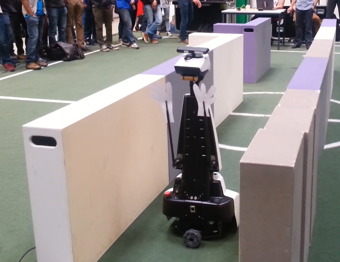
The image below links to a youtube video of the Corridor Challenge, in which we obtained a 3rd (19 seconds) place.

Final maze challenge

The final maze challenge was held at the 17th of July. During this challenge the hard work of 10 groups was put to the test to see which groups were able to finish the maze. Each group was allowed to make two attempts at solving the maze. The maze consisted of relatively standard part containing a loop, with a branch that lead to a door. Behind this door was a short corridor followed by an open space with a wall in the middle. at the other end of the open space the exit was situated.

Strategy

For the final maze challenge we had two versions of the code:

• Version 1: A version that partly relied on code that was tested before. However some changes were made after the last testing session, consisting of an updated motion skill section that chose a different alignment error when an open space was detected. This would result in wall-following in open spaces. Furthermore a basic solving strategy was implemented using the right-hand rule with an added loop detection feature. This way the robot would be able to break a loop in the maze by not choosing the rightmost branch if it detected a loop based on odometry data.

• Version 2: A safer version that originated form the last testing session. No loop detection was present and handling open spaces was not ideal.

What went wrong?

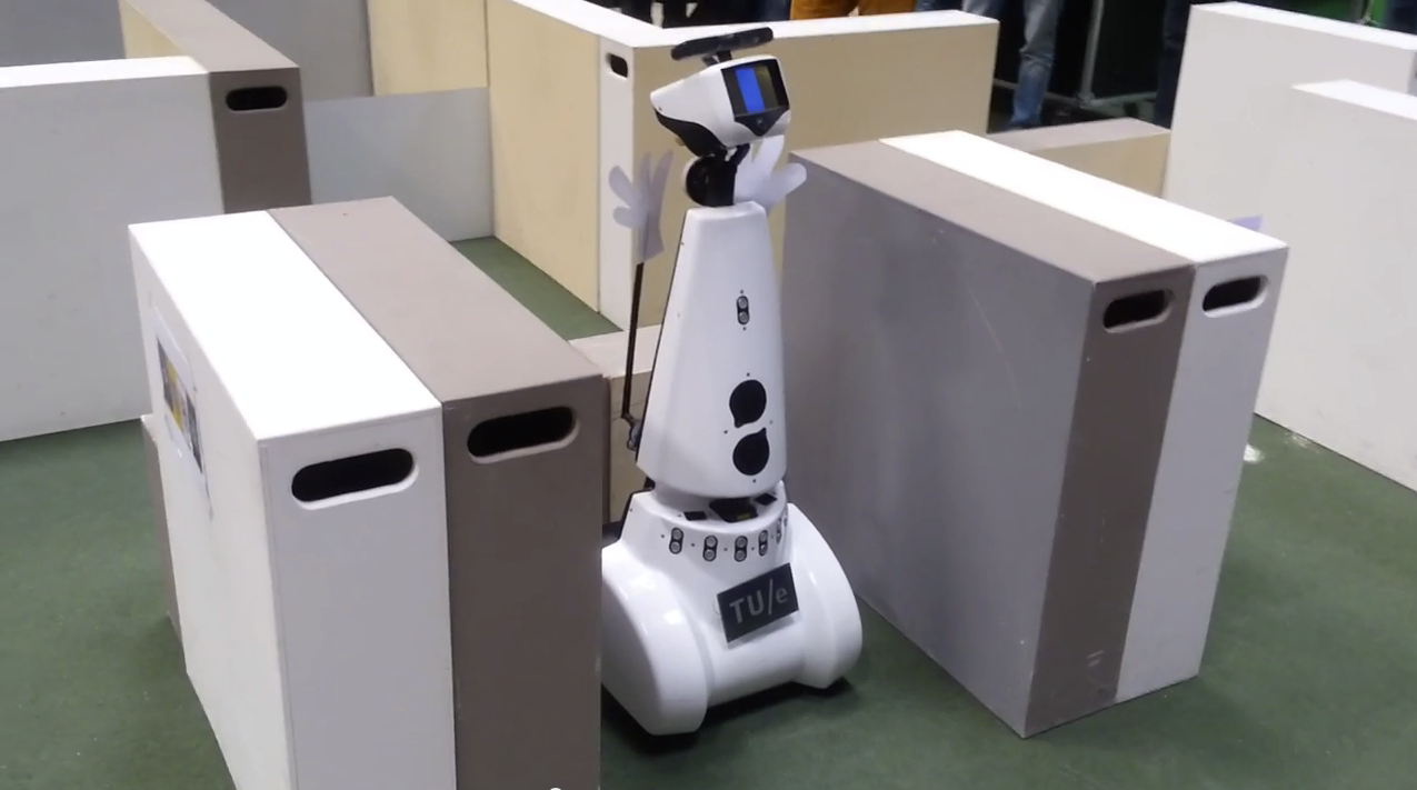
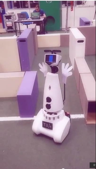
The video below shows the two trials. Clearly we did not finish the maze and did not even make it to the door. Both versions of the software detected a possibility to go right where there was none. After diving into the code we encountered the source of the bug. The laservision code had multiple ways of communicating the junction semantics to the supervisor. One was was through junction type integers and the other was through booleans for {left, right,front}. The latter functionality was however not updated in later versions since the laservision department assumed that the type codes would be used. This was a miscommunication that unfortunately led to the bug we see in the video.

Learning experiences

• Structure
  • Original design
  • Maintainable, scalable software
  • Applicable to future designs
• Communication
  • Unambiguous communication between developers
  • Using “standards”
• Prioritizing requirements
  • Essential vs. nice-to-have
  • Limited test time -> use cases
• C++ programming in Linux
  • Hands-on introduction in software development, GIT
  • Software development costs time
  • Reliable software is just as essential as hardware
  • Well-documented, well designed software is important