Embedded Motion Control 2015 Group 4: Difference between revisions
No edit summary |
|||
| Line 117: | Line 117: | ||
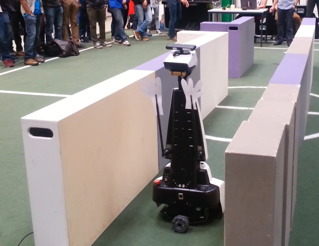
=Corridor Challenge= | =Corridor Challenge= | ||
[[File: | {| | ||
|[[File:emc2015_cor_gr4.jpg|center|250px|link=https://https://www.youtube.com/watch?v=hsuXMU-v9Os]] | |||
|} | |||
Revision as of 13:37, 25 May 2015
Authors: T. Cornelissen, T van Bommel, J. H. de Kleuver, M. Oligschläger, B. Hendrikx, P. Rooijakkers, T. Albers
Requirements and function specifications
Problem statement
The software design process starts with a statement of the problem. Although all the details of the assignment are not yet knwon at this point, we can best summarize the statement with the following sentence:
- Design the software in C/C++ for the (existing) Pico/Jazz robot that enables to find the exit of an unknown and dynamically changing maze in minimal time.
Requirements
A (draft) list of the requirements contains the following points:
- Exiting the maze in minimal time.
- Avoiding damage of the robot and the environment.
- Robustness of pathfinding algorithm with respect to maze layout.
- Design software using modular approach.
- Implement algorithm using only available hardware and software API's.
- Manage code development with multiple developers.
Existing hardware interfaces
- The Pico/Jazz robot with customized inner workings and a robot operating system with C++ API's.
- A (still unknown) wheelbase layout of which the possible DoF/turning radius is a design constraint.
- A lasersensor and acoustic sensor of which the range-of-visibility is a design constraint.
Unknown design constraints
- Simulation environment for code testing?
- Location of sensors and wheels relative to robot fixed frame?
- What data can we extract form the sensors?
- What does the maze look like? How do the doors operate?
Main focus point in the first two weeks
- Learn basics of C/C++ and software development.
- Determine the layout of the robot and the possibilities of the sensors and wheel structure.
- Become familiar with the integrated development environment.
- Explore the possibilities of th API's (how much postprocessing of the aquired sensor data is necessary and what techniques must be learned?).
Software design strategy
The figure below shows the overview of a posible software layout. The skill functions can be assigned to different programmers that are also responsible for exploring the API's and gathering details about the hardware. The maze solving strategy can be handled separately and the supervisory controller is the brain of the robot combining all the information. File:Maze example.pdf
Laser vision
Compass function
This function measures the angular misalignment of the robot with it's environment. The compass function gives a valid estimate of the angular misalignment under the following assumptions.
Assumptions:
- The world consists of mainly straight lines.
- All the lines cross each-other approximately with an angle which is a multiple of the world angle (when for example all the angles are perpendicular then the is 90 degrees)
- The current misalignment of the robot with it's environment is small: [math]\displaystyle{ \theta_{robot}\lt \lt 0.5\cdot\theta_{world\,angle} }[/math]. This implies that the compass function is unreliable during large rotations.
- There are enough sample points (preferably in front of the robot) to ensure that lines can be detected in the so called trust area.
- The trust area is defined as a bounded square around the robot which is aligned with the robot frame. Only the samples in this square are used for the compass function calculations. As is shown in the figure below.


Approach:
We are searching for a reference line from which we can calculate the angular misalignment of the robot. This calculation proceeds in the following sequence: First the laser data is expressed in a orthogonal frame (fixed to the robot). A line through point [math]\displaystyle{ [x_i,y_i] }[/math] can be described in polar coordinates as [math]\displaystyle{ p(\alpha)=x_i \cos(\alpha)+y_i \sin(\alpha) }[/math] where [math]\displaystyle{ p }[/math] and [math]\displaystyle{ \alpha }[/math] are unknown parameters. We want to find a [math]\displaystyle{ \alpha\in[0,\pi] }[/math] and a [math]\displaystyle{ p\in [-p_{max},p_{max}] }[/math] where [math]\displaystyle{ p_{max}=\sqrt{(2\cdot trust\,area\,size)^2} }[/math] is half the trust area diagonal. The Hough transform [1] gives a procedure to find [math]\displaystyle{ p }[/math] and [math]\displaystyle{ \alpha }[/math]. The procedure is as follows: for each [math]\displaystyle{ [x_i,y_i] }[/math] in the trust area and [math]\displaystyle{ \alpha\in[0,\pi] }[/math] the value of [math]\displaystyle{ p(\alpha) }[/math] is calculated.
The calculated [math]\displaystyle{ p }[/math] values are round to the closest value in a discrete set. The Hough parameter space can in this case be interpreted as a 2 dimensional grid where the first axis represents the value of [math]\displaystyle{ \alpha }[/math] and the second axis the [math]\displaystyle{ p }[/math] value, where for each solution of [math]\displaystyle{ p }[/math] a value of one is added to the corresponding cell in the grid. The parameters of our reference line are the parameters that corresponds to the highest value in the Hough parameter grid.
The Hough transformation is shown in the following figure. The x and y values of the laser measurements are shown on the left. On the right the Hough space is shown, where the red line represents the current [math]\displaystyle{ \alpha }[/math] value of our reference line.

Only the [math]\displaystyle{ \alpha }[/math] parameter is in this case of interest. Since we assumed that the angular error of the robot with its environment is small we calculate the misalignment as the smallest difference between the parameter [math]\displaystyle{ \alpha }[/math] and a multiple of the world angle (in other words it does not matter for the result when we find a reference line parallel to the robot y axis instead of a line parallel to the y axis).
Applications:
The result of the compass function can be directly used to reduce the angular misalignment of the robot with its environment. This is accomplished in the form of a simple gain feedback control rule: [math]\displaystyle{ \omega_z=K_ze_z }[/math] where [math]\displaystyle{ \omega_z }[/math] is the rotation velocity, [math]\displaystyle{ K_z }[/math] is a control gain and [math]\displaystyle{ e_z }[/math] is the angular misalignment found by this function. The other application of the compass function is to align the mini map with the robot’s environment.
Minimap
This function creates from the sample data a small map around the robot. The map indicates areas where obstacles are and where not. The purpose of the mini map is to make it possible for sub functions to simply and flexibly detect maze futures such as side paths, maze exits and position errors it forms also an important input for the world model.
The following points are of interest in this function:
Assumed in the compass function was that the angular misalignment is small and will converge to zero since it will be compensated by a controller. Therefore we align the mini map not with the robot frame but with the world. A second trust area is created, which forms the bounds of the mini map (with different dimensions as in the compass function). The map is discretized in blocks of a specified size (x-y accuracy in [m]).

In the figure above is shown:
- In A. the laser range finder data is transformed to a orthogonal frame:[math]\displaystyle{ x_i=r_i\cos(\theta_i) }[/math] and [math]\displaystyle{ y_i=r_i\sin(\theta_i) }[/math]
where [math]\displaystyle{ \theta_i=\theta_{increment}i+\theta_{min}-e_z }[/math]. - In B each sample i is fit in a block and when there is a sample in the block then the block/pixel value is changed to 1. The remaining blocks are left 0.
- In C a collision detection is applied to detect areas where there are no obstacles. This is a simple line search for each angle from the middle (robot position) up to a block or the trust area border. This is done for all the angles in the range of laser range finder. The maximum allowed angular step is the angle that a rib of a block on the thrust area border makes.
- In D the final binary mini map is shown (the center cell represents the robot position).
In the figure below is the
Functions that make use of the mini map:
Y position error (center error in corridor)
The Y position error is the distance of the robot to the middle of the corridor. The approach is to calculate a left and a right bound in front of the robot (we don’t look sideward but in front of the robot). From these bounds the following center error is calculated:
[math]\displaystyle{ e_y=\frac{k_{left}+k_{right}}{2} }[/math]
This center error is used to control the robot to the middle of the corridor with control rule: [math]\displaystyle{ v_y=K_ye_y }[/math]

Side path detection (as was used in the corridor challenge)
This function triggers when there is a side path found. The function calculates a front and a back bound. During the corridor challenge this function triggered the rotation function (which was tuned way to slow) under the conditions:
[math]\displaystyle{ |k_{front}|+|k_{back}|\gt minimal\,door\,size }[/math]
and
[math]\displaystyle{ |k_{back}|\gt |k_{front}| }[/math]

Exit detection (as was used in the corridor challenge)
If there is nothing in front of the robot then it is an exit.

Laser vision in action
In the figure below a simulation of the corridor challenge (third place, 19 seconds) is shown, it illustrates the robustness and simplicity of object detection in action. On the left the simulation of the robot trough the corridor is shown and on the right the mini map is shown.

Corridor Challenge
 |