Embedded Motion Control (EMC) Group 1 is a multidisciplinar and multilingual project group working on the 'A-MAZE-ING PICO'. This wikipedia page consists of the weelky progress presented in the #Journal, the written report and some other practical and useful stuff.

The report focussus on the individual components of the software architecture, this includes basic idea description, mathematical analyses and possible software implementation.

Journal

The proces of developing a software architecture and the implementation requires great coordination and collaboration. This journal will be updated to present and track the progress of the group. This journal includes weekly progress, countered problems and divided tasks.

Week 1

In the first week the overall process was discussed. Information from old groups were gathered and shared to clarify certain aspects and to get everyone in the group on the same level. The requirements, which were a selfstudy assignment, were setup using the FURPS (Functionality, Usability, Reliability, Performance, and Supportability) model in the meeting for the initial design report. Additionally, the installation of ubuntu and the relavant software were given as selfstudy assignments next to a division of tasks for the initial design report.

Week 2

In the second week the various role of System’s Architect, Team Leader, Secretary were defined. The team was split in pairs in order to approach the code development and the initial design document. Furthermore, deeper system’s description were identified and the software functions were made clearer using communication and context tasks.

Later in the same week the separately created system architectures (made by the earlier defined pair) were validated by discussing it in the meetings. Ideas on how to apply the 5C’s to low and low-level functionality were presented. Advantages and disadvantages on the use of potential fields were discussed. Tips were given by the tutor (in the first meeting with the tutor), with regards to the approach on the use of potential fields. Many practical stuff for the corridor challenge, were observed and identified with the help of the tutor.

For the self study assignments another division was created, to separately work on the report, presentation and the basics of the code, including potential field and low level functions. Additionally, the installation of Ubuntu, tools, software and simulators was given as mandatory assignments for everyone.

Week 3

After the long weekend, lasting through two-fifth of week 3, the presentation was given on Wednesday after which a meeting took place. A walk through of Git was done collaboratively in the group. The use of only the developing branch was decided upon for the development of the new algorithms. The master branch will just be used for final versions, supervised by the software architect. From that meeting until Friday's meeting codes were developed for the corridor challenge. Coordination of the tasks were maintained by the software architect.

Not everyone installed Ubuntu and all the tools yet, this created a lot of frustration for the other group members. The final deadline was set on 12:00 pm Wednesday.

Week 4

Over the weekend from week 3 to 4, majority of the coding related to Potential Field implementation was done. On Monday morning the first test run on PICO was done. Afterwards solutions for the cornering were discussed. And a proposal to have a hybrid solution between Potential Field and States-Decision were discussed. The State Machine consists of a Corridor Mode and an Intersection Mode.

For the code overview and explanation, the #Potential_Field and #Lower Level Skills are separately discussed. The results of the #Corridor Challenge are depicted later. After the corridor challenge, the group met to discuss the overall progress and the corresponding to do list and to do a quick intermediate evaluation of the group collaboration and the individual contribution thus far.

The following topics were discussed and divided as self study assignments:

Mapping strategy - To be defined during next meetings.
Decision Making - Refine behavior via updating parameters.
Improve Driving - Fine tuning the parameters for corridors and cornering.
Update Wiki
- Explanation of Safety Measurements.
- System Architecture.
- Videos from the simulators’ testing.
  - Big corridor + Potential Field
  - Previous stable versions of the system. Test them in simulator and get video.
    - Get positive and negative points from them. Analyze.
- Use of figures and diagrams explaining the methods.
- Potential Field grid (visualization).
- Explanation of our implementation of Potential Field.
- Minutes, meetings, requirements.
- Include time-based description of the project.
- Wiki Distribution
  - System Architecture (initial design)
  - Potential Field
  - Lower Level Skills
    - Drive
    - Safety Layer
  - Corridor Challenge Results
Clean up code - To be done in a new Branch
- Remove hard-coded stuff. Define possible new (and neat) states for current hacks.
- After cleaning up the code a new stable version (develop-2) should be available by next week.

Second Testing For PICO

The Second testing was done with the PICO for testing the bugs and the defects in the codes. It was found that the PICO moved well but It was not able to handle loops where it considered the loops as turnings that occur continuously, the reason for this was the mapping feature was not added to the code this problem was added later using the NODE approach discussed in the section Maze Mapping.

Week 5

Now the corridor challenge is successfully completed, we need to think about more advanced decision making, maze mapping, and a quicker turning skill. In week 5, not much coding was done, but several design ideas were thought through. The following components are thought through and coded in pseudocode:

Targeting correction: when a target is set in a new corridor, pico drives to it. However, that changes the target absolute position. A skill is created to cope with the absolute position, now a relative position is used, using odometry data to correct for it.
Node saving: to map the maze an array is used to store important points of interest. Containing: name, location, type of POI and linked POIs.
Visualization of targets: to debug the program a vizualization tool is created. All the information around PICO can be plotted separtetly while running the simulation.

MAZE MAPPING INITIAL APPROACH

Mapping the maze was an initial problem where the team decided to use different approach for mapping. After a long research and analysis using journals and websites that focuses on the LFR Mapping strategy, one of the team representative came up with the idea using SLAM (Simultaneous Localization and Mapping). It is a very popular method used to map the path of the LFR without using other sensor that has an high error rte. Its very robust and the signal to noise ratio is very high. So the error obtained can be minimized using filters. This method is very accurate compared to the odometer data. The LFR scans the area in a 2D plne. The local swept area is converted into a grid map that is represented by a DT (Distance Transform) Matrix. This is done using the LFR that considers the point where it meets the wall or an object as a value equivalent to '0'and, the other parts are considered as infinity and the values are stored in a matrix.

At the higher level the laser assigns distances from the wall to the LFR source with numbers to each position corresponding in a matrix using the function DT Matrix into T(X,Y,Φ) by linear simplex method.The DT matrix provides the information of each grid of a matrix with the Euclidean Distance to the nearest obstacle using the function DT(x,y)= min[(x-i)^2+(y-j)^2 => i=1, ……,M, J=1,…….,N]. M,N are the size of the matrix ( depends on the size of the path).

The Dt is transformed to x,y form of transformed matrix. Using the transfer function coding in C++ it is possible to convert the matrix in to coordinates.With the coordinates obtained it is easy to set the target in the half the range from it using the distance formula. then the PICO moves to that coordinate and the same process is done from that coordinate. The process is continuously repeated where the area scanned is mapped and stored in a stacked array. The turnings which is addressed by NODE in a junction is used to store the coordinate value using a seperate variable. This storage will enable the PICO to know the location of the turn and in case of loops it will enable it to know the coordinate where it was already there.

A simpler approach was also designed to make the decisions and keep the travk of the nodes named as the node approach was used, This is discussed in the section called as #Maze Mapping

Week 6

On Tuesday in the meeting the following desicions

Design Architecture

In this section, the initial idea of an embedded software design will be discussed. The main goal of the design is to make the Pico robot able to solve a maze. In this brief report, the requirements, functions, components specifications, and the interfaces of such a system will be discussed.

Requirements

The requirements of the system will be divided according to the FURPS model. The abbreviation of this model stands for Functionality, Usability, Reliability, Performance, and Supportability. Functionality in this case denotes the features and capabilities of the system. Usability includes the human factors, consistency, and aesthetics. Reliability stands for the failure frequency, accuracy, predictability, et cetera. Performance here means the efficiency, speed, response, i.e. measures of system performance. Finally, the supportability incorporates testability, maintainability, configurability, and so forth.

The main requirement of the system will be to navigate the maze. It must be completed according to the challenge specification, which forms the main functional aspect of the requirements.

Furthermore, the system design must be robust. The layout of the system must constitute all possible functions to account for the various system architecture, which enable the usability of that design. To achieve this, possible fault modes can be taken into account.

Also, the system design should pose a robust solution. This means the provided system solution must be robust enough to cope with the environmental uncertainties, so that the solution as a whole is reliable.

Next, the doors in the maze should be handled correctly. The behaviour of the door should be analysed to help differentiate the door from the wall. Firstly, the robot should be able to recognize a door from a wall and, secondly, cross the door.

Fifthly, the generated design should be tested for its reliability, and accordingly changes are required to be captured to improve the same.

Furthermore, The major functional requirement of the robot is the ability to solve the maze on its own.

Next, the given hardware (PICO robot) must be used for the maze challenge without any modification and additional components mounted on it.

Penultimately, the performance requirement of taking quick decision is one of the essential factors for the PICO robot for completing the challenge within 7 minutes.

And finally, the need for smart decision making is a crucial necessity due to the fact that the environment changes.

In the table below, the above requirements are summarized according to the FURPS structure.

**Summary of requirements according to the FURPS model.**
Requirement	F	U	R	P	S
Navigate the maze	x
Subsystem based design		x
Adaptable to environment			x
Door handling	x
Testing and simulation					x
Autonomous operation	x
Use given hardware		x
Fast decision making				x
Smart decision making				x

Functions

The functions of the system are classified according to three levels: high-level, mid-level, and low-level functionalities.

The high-level functionality incorporates the following three aspects:

Obtain relative position with respect to the global frame of reference in the maze.
Identification of the open or closed door.
Maze solving algorithm or strategy.

The mid-level functionality consists of:

Straight corridor navigation.
Collision avoidance algorithm.
Intersection mapping.

The low-level functionality contains:

The ability to read the laser and camera input.
Actuate the wheels according to the input.
System initialization for the working of the sensors and actuators.

Components

To obtain a clear overview of the system, its architecture is shown in the figure above, including its various components.

Specifications

The specifications of the system are formed by the available hardware and software, and by some of the requirements for the challenges.

Limited time to complete the maze challenge (7 min).
Limited access to the actual PICO robot.
Robot hardware is not to be modified.
Hardware access is facilitated via ROS.
Translational/rotational speed limit of the robot actuators.
Use of C++ and SVN.
Available sensors: Kinect and laser.
Use of controller feedback.
Unknown location of entrance and exit on the boundary of the maze.

Interfaces

Within the system, two types of interfaces are distinguished. First, there is the communication between the different components of the system, shown in the figure above as arrows. The second type of interface, is the interface on which the robot interacts with the environment. This includes a user interface to program the robot, and sensors to sense the environment. There is no user interface to communicate with the robot while it is solving the maze, for it is autonomous. The sensors used by the robot are discussed in the specifications.

Composition Pattern

Beside describing the behaviour of the model in a task-skill-motion model, an overview of the model structure can be made using composition patterns. A composition pattern describes the structure of the robot model focusing on a certain role. The composition pattern can be decoupled using the 5C's to develop functionality. The 5C's are the Computation, Communication, Coordination, Configuration and Composition of a certain part of the model. As an example of decoupling part of the composition pattern to develop functionality using the 5C's, the decoupling of the driving functionality will be explained.

Driving skill

Trigger??

To start the model

    when triggered % by OS, or other CP
     do {

Configuration

First the parameters are configured.

    speed = initial speed

Communication

Next, the computated Forcevector is communicated. This was calculated and is based on the decision of a target and the wall forces. Direction=GetForceVector

Coordination

Determine whether the target is in front of Pico, otherwise it should turn first.

   if |direction.angle| < 40
         drive forward
     else
          turn

Computation

Calculate the output speeds based on the coordinator decision and direction. For driving forward:

       speed = calculatetranslationalspeed

For turning :

       speed = calculaterotationalspeed

Scheduler

Now the speeds are determined, the driving can be scheduled.

       schedule() % now do one’s Behaviour

Communication

Send the scheduled speeds out to Pico.

       Pico.sendSpeed

Logging

       log()

Potentialfield

Trigger

To start the potentialfield, is should be triggered. The first time this will be done by constructing the world model, later on by updating the world model.

    when triggered % in world model
     do {

Configuration

The parameters of the potentialfield, the radius of the scanning circle are set.

    rangeCircle = 1.2  // Radius of the circle used for the potentialfield

Communication

Next, the potentialfield skill receives the laser data from Pico, by updating the class containing the laserdata.

       emc::LaserData * scan = pico->getScan();               // Get laser data

Coordination

Determine whether the target is in front of PICO, otherwise it should turn first.

   if |direction.angle| < 40
         drive forward
     else
          turn

Computation

Calculate the output speeds based on the coordinator decision and direction. For driving forward:

       speed = calculatetranslationalspeed

For turning :

       speed = calculaterotationalspeed

Scheduler

Now the speeds are determined, the driving can be scheduled.

       schedule() % now do one’s Behaviour

Communication

Send the scheduled speeds out to Pico.

       Pico.sendSpeed

Logging

       log()

Potential Field

In order to solve the maze successfully, the robot needs to be able to drive autonomously. This involves collision prevention and the ability to reach a certain target. While the target itself is provided by a higher level of control, we need some skill that actually reaches it. Our driving skill is able to do both by using a so-called resulting force vector. In principle, this system works quite easy. Objects and locations which are to be avoided have a repelling force, while desirable ones are given an attracting force. Then, the resulting force will give the most desirable direction to drive in, which only needs to be normalised and sent to the lowest level of drive control. For this to work, mathematically the function to calculate the force should be of a different order for undesirable and desirable targets, otherwise the robot could get stuck.

In practise, this is implemented as follows. For all wall points provided by the laser range finder, the following 'force' is calculated:

$[math]\displaystyle{ F_{w,i} = \frac{1}{r_m (r-0.05)^5}. }[/math]$

Of course, this gives numerical problems when the distance to the wall $[math]\displaystyle{ r=0.05 }[/math]$ . Then, a very high value is assigned. $[math]\displaystyle{ r_m }[/math]$ is a scaling constant, which can be tuned to reach the desirable behaviour later on. The contribution of each wall point in both in plane directions (x,y) is summed to obtain one force vector. Then, the target point is given force

$[math]\displaystyle{ F_t = r_t^2, }[/math]$

with $[math]\displaystyle{ r_t }[/math]$ the Euclidean distance to the target. The resulting force will be pointing in the direction which is most desirable to drive in. Note how this method is self regulatory, i.e. when the robot for some reason does not actually drive in the direction of the resulting force, the new resulting force of the subsequent time step will automatically correct for this. There is no need to store forces of all wall points, simply summing them vector wise will do. Also, there is no need for additional collision avoidance.

Add gif of force vector with walls and target. Add gif of pico driving.

Lower Level Skills

In this section, the lower level skills are elaborated on. Also, the implementation and the design decisions are explained.

Drive Skill

The Driving Skills are based on the information provided by the Potential Field and the higher level decision making. Once a target is set, the sum of the attracting force of the target and the repelling force of the walls will result in a net driving direction. This drive direction is scaled differently in the x and y direction with respect to Pico:

$[math]\displaystyle{ v_x = \frac{1}{2}\cos{(\theta)} v_{max} }[/math]$ ,

for the speed in x direction, where $[math]\displaystyle{ \theta }[/math]$ denotes the angle of the drive vector, and

$[math]\displaystyle{ v_y = \frac{1}{5}\sin{(\theta)} v_{max} }[/math]$

For the speed in the y direction. The rotational speed is simply 1.5 times the angle of the net driving direction vector. However, when the drive angle becomes larger than 40 degrees, we only rotate towards it to prevent collisions. Then, pico->setSpeed is updated. In Pico's low level safety layer, we have a safety built in that the robot is not allowed to move backwards. When the drive vector is pointed that way, we allow it only to rotate and move in the y direction.

Safety Layer

The first safety measure is the potential field algorithm itself. It's obvious that the robot should keep from getting too close to the walls. However, with regards to completeness and having safety redundancies in the code, another safety routine was implemented. The basic idea is to prevent the robot from hitting the walls (either head-on and/or otherwise), so the distance to the walls is continuously compared to a safety margin. If the distance is smaller the robot will stop and enter a routine that maneuvers the robot away from the wall and places the robot in a location to keep driving safely.

A second safety measure is the connection state skill. A true state of this skill is required to run the main loop, activating all the other skills and tasks of Pico. This is a very basic function, nevertheless, required for robust operation.

Sensor data acquisition

One of the low level skills is the interface with the hardware. Pico is equipped with a an Odometry sensor measuring the relative base movement and with a laser range finder, measuring distances. Both these hardware components can be individually activated as a low level skill. Other functions, skills, and tasks can use this globally available data.

Turn Skill

In order to have a modular approach to solving the side turns, the operations were separated using a simple state machine. When advancing through the corridor, the robot is checking for large magnitude differences between the laser's measurement vectors. These differences could represent an "opening" in the wall, which being large enough indicate a new corridor. If the robot detect that the corridor has two possible paths, the state is changed to "Junction" mode. Immediately after this information of "Junction" mode at this point in the maze a junction location will be stored. This information is not used for the turning itself, but could prove useful when designing the higher decision skills to solve the maze. Once the data is stored, the current state will be "Drive Junction", which takes the robot to an estimate of the junction's center. At this point, the robot will turn to whichever side the new corridor is. These states are represented graphically in the following figures.

Once the robot has taken a turn it must enter the new corridor, detect the walls so that it can continue navigating in the new corridor. Such operations are carried out by a "Drive Out" state. If the laser signal indicates that the robot is again in a corridor it moves back to the "Navigate Corridor" state and continues. When the robot detects that there are no more walls in front of it and on the sides, and there are no large differences between the laser vectors (implying, there are no new corridors), its interpretation is that the corridor challenge has been completed. So a "Victory" state is reached that will stop the robot's motion. The next figure shows these states.

Corridor Challenge

Preparation of the Embedded Motion Control #Corridor Competition and the results shown in a short movie.

Available Approaches

Based on the results from the test run with the real robot, the following solutions were proposed: Robust Turning. Safe or Fast modes. Simple Turns. Hard-coded turns.

A relevant concept in the development of the solutions was to be able to identify that the robot was turning and not only turn as an extension of "regular corridor driving". As a result, a simple state machine was implemented. It modifies the decision making of the robot as long as it recognizes to be in a turn.

Results

The driving through the straight part of the corridor was smooth and fast reactions were not evident. Just as in the simulation shown previously, the robot detected the side exit appropriately.

The separation of the turning action into states is meant to facilitate the implementation of higher level navigation afterwards. After the challenge some new scenarios were tested to gain some insight of the robustness of the code. First, a small separation between the wall-blocks. Second, narrower corridor. And finally, remove the side exit walls to check if the robot could still recognize it, turn and stop. From these new scenarios, the results were as follow: 1) the code is able to navigate well even is some discontinuities exist in the walls, 2) The robot can drive through the corridor regardless of it having a different width, however, if the width is smaller than the safety margin established in the code, the robot will not move. And 3) Even if the side-corridor has no walls the robot was able to recognize it, turn and stop. These tests show that the robust approach can deal with an uncertain environment up to this level.

Maze Challenge

After a discussion within the team on the approach for the maze challenge, a high-level logic was defined. The basic idea is presented in the following Figure:

These three steps have several implications on a lower level. For example, one of the main difficulties is how will the robot gain knowledge about the maze. Being able to know that the robot has been in a given section of the maze before, and also knowing if there is a possibility that has not been tried yet in a given junction.

Training Maze Description

The scenarios that can be faced during the final challenge are diverse. Therefore, various maze design were constructed having specific properties to enable the identification of robustness of PICO for navigating through specific type of maze. The following specific types of maze for testing the robustness of PICO is as shown below:

This particular maze checks the wall, T-Junction and Open Space handling capability of PICO.

This maze is responsible for making sure that PICO is able to handle the gross and thin walls alike, ans also Dead Ends and Open Spaces.

Based on the description from the course's Wiki the test maze of the following Figure was designed.

File:Edited Maze .png

It has multiple dead-ends, T junctions, X junctions and several corners. It also has three different possible loops marked by the red, green and blue lines of the following Figure.

This first map contains sections which can be used to test a robust maze solving logic.

After getting through the inital mazes for the basic test of the robustness of PICO navigation, the ultimate maze was designed to push the limit for the PICO navigation, with the ultimate maze as shown below: -

Recognizing Maze Features

In order to be able to store maze features in some sort of map, there is a need to identify them using the laser data, preferably in the least number of steps to increase the performance of the algorithm. To achieve this, a robust and quick way to distinguish between the maze features has to be conceived. For the corridor challenge gap vectors were already built from the laser data, as was already explained before. Now, these features are extended with the wall vectors.

The main principle is as follows: From the laser data, the so called corner points are deducted (indicated in the figure referred as black circles). It is also noted that every maze feature has a unique number of corner points. For instance, a simple corner has only one, and a full junction 4. Then, by counting both the wall vectors and the corner points, every feature can be robustly identified.

Maze Mapping

The question the becomes, how to build the world model? Starting with the premise of building a simplified model having only the information necessary to solve the maze. The approach proposed is to use nodes, which represent relevant features from the maze, e.g. start and end points, different kinds of junctions, corners and open areas. Relevant characteristics to be saved are the approximated global position of each node and how it is connected to the nodes around it. The following Figure shows a rough representation of a simple maze loop.

A very relevant problem to be solved is that of "loop closure", so that the robot can navigate smartly through the maze without repeating corridors if unnecessary. After discussing this problems with the team, the following characteristics were selected as the most relevant:

Node identification number.
Node type, e.g. start, T/X junction, dead end, open area, corner, end.
Movement direction referenced to initial robot orientation.
Connected nodes.

Node Approach

The conditions for the state machine were observed, identified and storing the Junction properties in the nodes was implemented. The properties of the Junctions which are stored in the nodes are as follows: -

Identification Number - Unique for each node.
Type - The type of the Junction encountered.
History - Whether the particular node was visited by the PICO while mapping the maze

Detection of Dead Ends

The detection of dead ends was done on the basis of comparing with the number of targets which are basically the gap vectors and therefore determining the effective available gap or a dead end. If there are no gaps detected and/or one target detected which is close to PICO, then a deadend has been reached.

Detection of Open Space

The open spaces are detected basically using the range circle which is made wider and broader, depending on the number of gap vectors detected using the 5 global iterations, the minimum gap is determined and accordingly the identification of open space is performed.

Decision State Flow

The high level navigation algorithm was constructed as a state machine. One of the main assumptions is that the robot will always start in a corridor, as such, the initial state of the diagram is "Junction". For a quick overview the following figure is presented:

Here, it is possible to see that the information required for most of the state transitions is the number of gaps and in few cases a new check on the laser data.

The groups of states including "Junction", "Drive Junction", "Store Junction" and "Drive out Junction" are used for the junction navigation. So, in terms of physical meaning inside the maze, they are all located in the different kinds of crossings.

Maze Competition

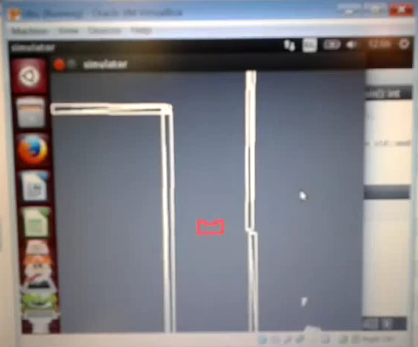
Before the maze competition the system was tested in the simulator and in the laboratory. The simulator was mainly used to check high level logic, such as recognizing intersections, turning, recognizing dead ends and following the door routine. The following video shows a simulation with the robot navigating a cross junction map with a door in one of the corridors.

Unfortunately the robot was not able to finish the Maze Challenge. Therefore, the team decided to reproduce the design of the maze in the simulator to test the system used on the day of the competition. The resulting maze can be seen in this illustration:

The robot was then able to navigate through the first section of the maze, find and cross the door. Cross the open space after the door and approach the zone where the exit was finally located. Before actually going to the exit, a problem with the open space identification emerged, therefore the system did not know what to do and started switching between states very fast. This all can be seen in the next video:

Uniqueness of the Design

     The implementation of the potential field methods to find the optimal path for the robot (PICO) is one of the best methods implemented by the group. With this the robot can detect walls very easily and maneuver on the path provided. The potential field method is used in many arduino robots. It is considered as the most robust technology in object identification. The potential field is developed by the laser scanning (LFR) and it allots potential of low and high levels for free paths and walls. The walls get a high potential so the robot knows that there is an obstacle.
The state machine approach allowed PICO to map the maze features and navigate accordingly. The Potential Field was particularly helpful in letting PICO make decisions based on the targets set in the maze, while the state machine approach let PICO identify the maze and take decisions based on this information. 
A simple and deft decision design or algorithm was developed where the PICO makes decision random in a random choice. this increases the probability of making decisions for turning in different directions. Another advantage of this algorithm is that it helps in the prevention of loops. So it is considered as the best methods to avoid the PICO from looping the maze.

Problems encountered and their counter measures

Appendix

References

Website References

   [1] http://www.instructables.com/id/Maze-Solving-Robot/
   [2] http://letsmakerobots.com/node/37746
   [3] http://onlinelibrary.wiley.com/journal/10.1002/(ISSN)1099-1514
   [4] http://www.researchgate.net/journal/0143-2087_Optimal_Control_Applications_and_Methods
   [5] http://blog.miguelgrinberg.com/post/building-an-arduino-robot-part-ii-programming-the-arduino
   [6] http://robotics.stackexchange.com/questions/1544/arduino-c-c-progamming-tutorials
   [7] http://www.robotshop.com/blog/en/how-to-make-a-robot-lesson-10-programming-your-robot-2-3627
   [8] http://cstwiki.wtb.tue.nl
   [9] http://www.instructables.com/id/Simple-Arduino-Robotics-Platform/
  [10] http://www.cplusplus.com/doc/tutorial/
  [11] http://www.tutorialspoint.com/cplusplus/
  [12] http://www.cprogramming.com/tutorial.html
  [13] http://letsmakerobots.com/artificial-potential-field-approach-and-its-problems

Journal and Hard Copy References

   [1] Airborne laser scanning—an introduction and overview Aloysius Wehr & Uwe Lohr,ISPRS Journal of Photogrammetry & Remote Sensing 54 1999 68–   
       82
   [2] Bachman, Chr. G., 1979. Laser Radar Systems and Techniques. Artech House, MA.
   [3] Baltsavias, E.P., 1999. Airborne laser scanning: existing systems and firms and other resources. ISPRS Journal of Photogrammetry and    
       Remote Sensing 54 2–3 , 164–198, this issue.       
   [4] Young, M., 1986. Optics and Lasers—Series in Optical Sciences. Springer, Berlin, p. 145.
   [5] Airborne laser scanning—present status and future expectations,ISPRS Journal of Photogrammetry & Remote Sensing 54 1999 64–67
   [6] http://www.robotshop.com/media/files/pdf/making-robots-with-arduino.pdf
   [7] Design and Development of a Competitive Low-Cost Robot Arm with Four Degrees of Freedom Modern Mechanical Engineering, 2011, 1, 47-55
       doi:10.4236/mme.2011.12007 Published Online November 2011 (http://www.SciRP.org/journal/mme) 
   [8] Semantic World Modelling for Autonomous Robots, Jos Elfring

Group members

Group 1 consists of the following members:

Name	Student nr	Email
Maurice Poot	0782270	m.m.poot@student.tue.nl
Timo Ravensbergen	0782767	t.ravensbergen@student.tue.nl
Bart Linssen	0786201	a.j.m.linssen@student.tue.nl
Rinus Hoogesteger	0757249	m.m.hoogesteger@student.tue.nl
Nitish Rao	0927795	n.rao@student.tue.nl
Aakash Amul	0923321	a.v.h.amul@student.tue.nl
Ignacio Vazquez	0871475	i.s.vazquez.rodarte@student.tue.nl

Qt from terminal

If Qt Creator is not run from the terminal, the programs inside cannot connect to the ROS master. To be able to run Qt Creator from the desktop without any problems, follow a similar procedure to the one that is used in the Customizing Ubuntu tutorial for the Terminator file:

Edit

~/.local/share/applications/QtProject-qtcreator.desktop

and change the third line to:

Exec=bash -i -c /home/rinus/qtcreator-3.3.2/bin/qtcreator

This will run QtCreator from a terminal even if the desktop icon is used.

Embedded Motion Control 2015 Group 1

Journal

Week 1

Week 2

Week 3

Week 4

Second Testing For PICO

Week 5

Week 6

Design Architecture

Requirements

Functions

Components

Specifications

Interfaces

Composition Pattern

Driving skill

Trigger??

Configuration

Communication

Coordination

Computation

Scheduler

Communication

Logging

Potentialfield

Trigger

Configuration

Communication

Coordination

Computation

Scheduler

Communication

Logging

Potential Field

Lower Level Skills

Drive Skill

Safety Layer

Sensor data acquisition

Turn Skill

Corridor Challenge

Maze Challenge

Training Maze Description

Recognizing Maze Features

Maze Mapping

Node Approach

Detection of Dead Ends

Detection of Open Space

Decision State Flow

Maze Competition

Uniqueness of the Design

Problems encountered and their counter measures

Appendix

References

Group members

Qt from terminal

Navigation menu

Search