Embedded Motion Control 2014 Group 2

Members of Group 2:

Michiel Francke

Sebastiaan van den Eijnden

Rick Graafmans

Bas van Aert

Lars Huijben

Planning:

Week1

• Lecture

Week2

• Understanding C++ and Ros
• Practicing with pico and the simulator
• Lecture

Week3

• Start with the corridor competition
  • Start thinking about the hierarchy of the system (nodes, inputs/outputs etc.)
  • Dividing the work
    • Driving straight through a corridor
    • Making a turn through a predefined exit
    • Making a turn through a random exit (geometry unknown)
• Meeting with the tutor (Friday 9 May 10:45 am)
• Lecture

Week4

• Finishing corridor competition
• Start working on the maze challenge
  • Think about hierarchy of the system
  • Make a flowchart
  • Divide work
• Corridor challenge

Week5

• Continue working on the maze challenge

Week9

• Final competition

Corridor Challenge

Ros-nodes and function structure

The system for the corridor challenge is made up from 2 nodes. The first one is a very big node which does everything needed for the challenge, driving straight, look for corners, turning, etc. The second one is some kind of fail-safe node which checks for (near) collisions with walls and if so, it will override the first node to prevent collisions. The figure next to the ros-node overview displays the internal functions in the drive-node.

Each time the LaserCallBack function gets called the CheckWalls function is called in it. This function looks at the laser range at -pi/2 and pi/2. If both the lasers are within a preset threshold it sets the switch that follows the CheckWalls function such that it will execute the Drive_Straight function. If either the left or the right laser exceed the threshold it will cause the switch to execute the Turn_Left or Turn_Right function respectively. If both lasers exceed the threshold pico must be at the exit of the corridor and the stop function is called. Each of these functions in the switch set the x,y and z velocities to appropriate levels in a velocity command which can then be transmitted to the velocity ros-node.

Corridor challenge procedure

The figures below display how all the different functions in the switch operate and it also shows the general procedure that pico will follow when it solves the corridor competition.

Action 1: In the first picture we see pico in the drive straight mode. The lasers at -pi/2 and pi/2 are being monitered (indicated in black) and compared with the laser points that are closest to pico on the left and right side (indicated with red arrows). The y-error can now be interpreted as the difference in distance between the two red arrows divided by 2. The error in rotation can be seen as the angle difference between the black and red arrows. In order to stay on track pico magnifies the y and theta errors by a negative gain and sends the resulting values as the velocity commands for the y and theta velocity commands respectively. This way pico is always centered and aligned with the walls. The x-velocity is always just a fixed value.

Action 2: As soon as pico encounters an exit, one of its lasers located on the sides will exceed the threshold causing the switch to go to one of the turn cases.

Action 3: Once in the turn case, pico must first determine the distance to the first corner. This is being done by looking at all the points in a set field of view (the grey field) and then determining which laser is the closest to pico. The accompanying distance is stored as the turning radius and the accompanying integer that represents the number of the laser point is stored as well. For the second corner we do something similar but look in a different area of the lasers (the green field), again the distance and integer that represent the closest laser point are stored.

After this initial iteration, each following iteration will relocate the two corner points by looking in a field around the two stored laser points that used to be the closest to the two corners. The integers of the laser points that are now closest to pico and thus indicate the corners, are stored again such that the corner points can be determined again in the following iteration.

The distance towards the closest point is now being compared with the initial stored turning radius, the difference is the y-error and is again magnified with a negative gain to form the y-speed command. The z-error is determined from the angle that the closest laser has with respect to pico, this angle should be perpendicular to the x-axis of pico. Again the error is magnified with a negative gain and returned as the rotational velocity command. This way the x-axis of pico will always be perpendicular to the turning radius and through the y correction we also ensure that the radius stays the same (unless the opposing wall gets to close). The speed in x-direction is set to a fixed value again, but it only moves in x-direction if the y and z errors are within certain bounds. Furthermore, also the y-speed isn't enforced if the z error is too large. This in this order we first make sure that the angle of pico is correct, than we compensate for any radius deviations and finally pico is allowed to move forward along the turning radius.

Action 4: If pico is in the turning case, the checkwalls function is disabled and the routine will always skip to the turn command, thus an exit condition within the turning function is required. This is where the tracking of the second corner comes in. The angle [math]\displaystyle{ \varphi }[/math] that represents the angle between the second corner and one of the sides of pico is constantly being updated. If the angle becomes zero, pico is considered to be done turning and should be located in the exit lane. The turning case is now aborted and pico should aromatically go back into the drive straight function because the checkwalls function is reactivated.

Action 5: Both the left and right laser exceed the threshold and thus pico must be outside of the corridor's exit. The checkwalls function will call the stop command and the corridor routine is finished.

Note: If the opposing wall would be closed (an L-shaped corner instead of the depicted T-shape) the turning algorithm will still work correctly.

Corridor competition evaluation

We achieved the second fastest time of 18.8 seconds in the corridor competition. Our scripts functioned exactly the way they should have. However our entire group was unaware of the speed limitation of 0.2 m/s (and yes we all attended the lectures). Therefore, we unintentionally went faster than we were allowed (0.3 m/s). Nevertheless, we are very proud on our result and hopefully the instructions for the maze competition will be made more clear and complete.

Maze Competition

Flowchart

Our strategy for solving the maze is shown schematicallly in the figure below. The strategy used here differs from the strategy used in the corridor competition. Now we create a map of the surroundings with pico's laser data. This map gets updated and new information will be added when pico drives through the world resulting in a detailed overview of the complete area. This enables us to remember the places pico has visited and to make smart choices while solving the maze. Furthermore, due to the approximated position of walls in the map we are less dependent on the latest sensory data. We are able to anticipate on upcoming crossings, deadends and plan relatively simple trajectories.

Six nodes ( Arrow detector, Hector mapping, Map interpreter, case creator, top level decision and trajectory) have been developed and communicate with each other through several topics. The nodes are subscribed on topics to receive sensory data coming from the laser, camera and odometry modules. All nodes are launched in one launch file. The function of the individual nodes will be discussed below.

Determine cases

Dead end detection

During Pico's route through the maze dead ends will be encountered. Obviously, driving into a dead end should be avoided to keep the journey time to a minimum. If Pico is arrived on the center of a crossing a clear overview of situation will become visible in the map. This situation is depicted in the figure below.

For a maximum of three crossingexits (depending on crossing type) will be checked if the corresponding corridor results in a dead end. From the map interpreter which interprets the hector mapping node, the walls (lines) are known in absolute coordinates (indicated with a start and end point). In the dead end function first all lines that lay on the four check points of the current crossing will be searched for in the array where all lines are stored. So for the figure above, first for the lower left (LLT) corner point and upper left (ULT) corner point, then for ULT corner point and upper right (URT) corner point and finally for URT corner point and lower right (LRT) corner point the dead end will be checked. For example, for the exit above will be checked if line C gets intersected twice this is the case (lines A and B).

Decision

The top level decision node decides in which direction a trajectory should be planned. It finds a new set point which becomes a target point for the trajectory node. The top level decision node is subscribed to four topics. First of all it is connected to the odometry module and secondly to Hector mapping node to receive information to determine the current position of pico. Furthermore, it is subscribed on a topic which is connected to the arrow detector node. The arrow detector node as will be described in the next paragraph sends a integer message 1 for a left arrow and 2 for a right arrow to help pico find the correct direction. Two major situations can be distinguished in this node and are depicted below in the figures:

1. A turn can be initiated before the crossing [type 1 or type 2]

From the case creator node follows that a simple corner (of type 1 or 2) is nearby. A starting point and endpoint are placed (green points in figure) so pico does not have to reach the center of the crossing first. Then a curved trajectory can be planned in the next node. Besides the x- and y coordinates of these two points also the type of corner (left or right) and coordinates of the turning point (lower left corner) are send in a float32mulitArray message to the trajectory node.

2. Go to center of crossing for overview of situation [ type 3, type 4, type 5 or 6]

For all the other types of crossings all the sides have to be checked if going that direction will result in a deadend. In a type 5 situation (T-crossing) with arrow information, the choice will be based on the direction of the arrow. If no arrow is present (or detected) a random function will be called to decide whether to go left or right. If it is possible to go foward that will always be the preferred direction.

Trajectory

For letting Pico drive in the right directions through the maze, a trajectory node is made. With means of Hector Mapping, Pico’s laserdata is converted to a virtual map of the maze. In general, it is possible to determine Pico’s location from the (interpreted) map, however the update frequency of Hector Mapping is only a 0.5 Hz. Therefore, pico’s location is besides hector mapping also determined by the data from the odometry topic. This topic sends the actual orientation of Pico with respect to a base frame which has its origin at the initial starting point of Pico. It could be possible however that this base frame does not coincide with the base frame of the map made by Hector Mapping. Therefore the odometry data has to be corrected every time a new map is published. This way the coordinate frames of the map and the Odometry data will coincide.

Now that Pico knows its orientation within the map, it can orient its way to a new desired location. This location is specified by the high level decision node. Depending on the geometry of the maze, the trajectory from Pico’s actual position to the newly specified location could either be a straight line, a curve to the left or a curve to the right. The type of trajectory is specified in the message published by the high level decision node with means of an integer (0,1 or 2). Next, depending on the type of trajectory, the trajectory will be discretized in a number of points and pico will move in a straight line between these discretized points, as is also shown by the yellow temporary points in the figures above.

Straight line

With means of Pythagoras’ theorem the absolute distance between the start and end point is calculated. This distance is divided into a certain number of points with equal length L. The angle between the two points (\theta) is calculated relative to the Hector Mapping frame. Now the set of coordinates between the two points can be calculated in a for loop by adding (or subtracting) i*L*sin(\theta) to the x coordinate and i*L*cos(\theta) to the y coordinate of the starting point.

Curve

Discretized ellipsoid-like turn

It is possible that the corridors in the maze do not all have the same width. Therefore, it is not suitable to make a perfect circular arc for making the turn. Otherwise pico will not end up in the middle of the new corridor. Actually, this is not a big problem because pico will automatically correct itself. But for a more robust routeplanning and to have a better flow through the maze it is better to make an ellipsoid-like turn. This is shown in the figure to the right. This will particularly be useful if corridor widths will differ substantially.

The discretization of the trajectory will be done in theta, as defined in the figure. To convert theta to the useful coordinates x and y, the radius is computed for each point and subsequently the x and y coordinates are computed using basic goniometry. The radius for an ellipse is given by,

[math]\displaystyle{ r(\theta)=\frac{ab}{\sqrt{(b \cos{\theta})^2+(a \sin{\theta})^2}} }[/math]

Thresholds

Now that the vector of points is constructed, Pico can drive from a point to an upfollowing point in that vector to eventually reach the desired end point. For smooth and correct driving, it is necessary that Pico’s orientation is always parallel to the trajectory. This means that Pico must always ‘look’ towards the next point in the vector. To achieve this the angle between the two points (target_angle) with respect to the Hector Mapping base frame is calculated. An angular velocity is send to Pico to let it turn in the right direction. The target_angle is constantly compared to the actual orientation of pico (actual_angle). If it now holds that abs(target_angle – actual_angle) < threshold, the angular velocity is set to 0.0.

Similarly, pico will never reach the exact target position. Analogously to the target angle a threshold system for the position is made to define when pico has reached a new point. This system looks something like abs(target_pos.x-actual_pos.x)<threshold && abs(target_pos.y-actual_pos.y)<threshold.

Arrow detection

Although the arrow detection is not crucial for finding the exit of the maze, it will potentially save a lot of time by avoiding dead ends. That is why we considered the arrow detection as an important part of the problem, instead of just something extra. The cpp file provided in the demo_opencv package is used as a basis to tackle the problem. The idea is to receive ros rgb images, convert them to opencv images (.mat), convert them to hsv images, find 'red' pixels using predefined thresholds, apply some filters and detect the arrow. The conversions are applied using the file provided in demo_opencv, but finding 'red' pixels is done differently.

Thresholded image

Opencv has a function called InRange to find pixels within the specified thresholds for h, s and v. To determine the thresholds, one should know something about hsv images. An hsv image stands for hue, saturation and value. In opencv the hue ranges from 0 to 179. However the color red wraps around these values, see figure a.1. In other words, the color red can be defined as hue 0 to 10 and 169 to 179. The opencv function InRange is not capable of dealing with this wrapping property and therefore it is not suitable to detect 'red' pixels. To tackle this problem, we made our own InRange function, with the appropriate name 'InRange2'. This function accepts negative minimum thresholds for hue. For example:

min_vals=(-10, 200, 200);
max_vals=(10, 255, 255);
inRange2(img_hsv, min_vals, max_vals, img_binary);

Makes every pixel in img_binary for which the corresponding pixel in img_hsv lies within the range [H(169:179 and 0:10) S(200:255) V(200:255)] white and otherwise black. This results in a binary image (Thresholded image), see for example figure a.3 which is a thresholded image of figure a.2.

Filter

The thresholded image likely contains other 'red' clusters besides the arrow. A very basic filter is applied to filter out this noise. The filter computes the average x and y of all the white pixels in the thresholded images. Subsequently it deletes all the pixels outside a certain square from this average. The length and width of this square have a constant ratio (the x/y ratio of the arrow ~ 2.1) and the size is a function of how many pixels are present in the thresholded image. This way the square becomes proportionally with the distance of the arrow. This approach is very prone to noise and therefore an additional safety is applied. The detection only starts if the number of pixels present in the filtered image lies between 2000 and 5000. These numbers are optimized for an arrow +- 0.3 to 1.0 meter away from pico. An example of the applied filter is shown in figure a.3. The red lines are the averages and everything outside the square is deleted.

detection

To detect whether the resulting image contains an arrow to the left or an arrow to the right, the following algorithm is used:

determine new means
compute standard deviations in terms of y for both halves of the picture. That is left and right of the average x (Sl and Sr)
If Sl-Sr>threshold ---> arrow left
If Sl-Sr<threshold ---> arrow right
else ---> no arrow detected

Of course, this method is not very robust and prone to noise. However, it is very efficient and it is able to detect arrows in the maze consistently.

• 

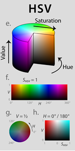
  Figure a.1

• 

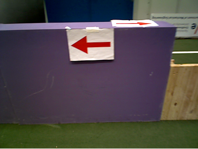
  Figure a.2

• 

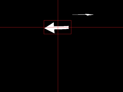
  Figure a.3

• 

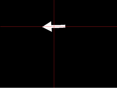
  Figure a.4

Time Survey Table 4K450

Members	Lectures [hr]	Group meetings [hr]	Mastering ROS and C++ [hr]	Preparing midterm assignment [hr]	Preparing final assignment [hr]	Wiki progress report [hr]	Other activities [hr]
Week 1
Lars	2	0	0	0	0	0	0
Sebastiaan	2	0	0	0	0	0	0
Michiel	2	0	0	0	0	0	0
Bas	2	0	0	0	0	0	0
Rick	2	0	0	0	0	0	0
Week 2
Lars	2	0	16	0	0	0	0
Sebastiaan	2	0	10	0	0	0	0
Michiel	2	0	8	0	0	0	0
Bas	2	0	12	0	0	0.5	0
Rick
Week 3
Lars	2	0.25	4	13	0	0	0
Sebastiaan	2	0.25	6	10	0	0	0
Michiel	2	0.25	6	2	0	0	0
Bas	2	0.25	4	10	0	0	0
Rick
Week 4
Lars	0	0	0	12	0	4	0
Sebastiaan	0	0	1	10	0	0	2
Michiel	0	0	0	2	10	2	0
Bas	0	0	0	13	0	0	0
Rick
Week 5
Lars	2	0	0	0	22	0	0
Sebastiaan	2	0	0	0	20	0	0
Michiel	0	0	0	0	16	0	0
Bas	2	0	0	0	14	0	0
Rick
Week 6
Lars	0	0	0	0	20	0.25	0
Sebastiaan	0	0	0	0	20	0	0
Michiel	0	0	0	0	20	0	0
Bas
Rick
Week 7
Lars
Sebastiaan	0	0	0	0	20	0	0
Michiel	0	0	0	0	20	0	0
Bas
Rick
Week 8
Lars
Sebastiaan
Michiel
Bas
Rick
Week 9
Lars
Sebastiaan
Michiel
Bas
Rick
Week 10
Lars
Sebastiaan
Michiel
Bas
Rick