Embedded Motion Control 2014 Group 12

Introduction

Members of group 12

Groupmembers (email all)
Name:	Student id:	Email:
Anthom van Rijn	0737682	e-mail Anthom
Jan Donkers	0724801	e-mail Jan
Jeroen Willems	0755833	e-mail Jeroen
Karel Drenth	0863408	e-mail Karel

Corridor Challenge

The goal of the corridor challenge is to make pico drive autonomously trhough a corridor, recognize a T-junction successfully, and have it take the appropriate corner.

Planning

Week 1

• First Lecture

Week 2

• C++ tutorials
• ROS tutorials
• SVN tutorials
• Run the first test on pico (safe_drive.cpp) to get some hands-on experience.

Week 3

• Start the actual coding, based on the safe_drive.cpp file. Paying special attention to robustness and exceptions.
• Have pico recognize situations (corridor, corner, t-junction,dead-end, etc.) and act accordingly
• Have the script succesfully run in simulation

Week 4

• Fine tuning of script
• Corridor Competition

Software Architecture

Initially, the choice was made to forgo the notion of speed and first create a robust algorithm that would successfully recognize a situation, using only the laser data, and take the appropriate action. The situations that should be recognized are depicted in table below. In this case, it's assumed that all junction/corners are right handed, although it works equally for left handed situations.

Situation recognition

Goal: to successfully recognize a situation and take the corresponding action.

Corridor challenge	Corridor challenge	Corridor challenge
Recognize a corridor (action: keep on driving)	Recognize the exit (keep on driving, then stop)	Recognize a corner (action: take the corner)
Recognize a corner (action: take the corner	Recognize a T-junction (action:take a right turn	Recognize a corner (action: take the corner

Robustness

As can be seen, it is important to calibrate the ranges of the laser data to make sure that the situation is evaluated correctly. If this is done wrong, the situation might be evaluated incorrectly and PICO might come to a halt (due to a hard constraint) and be unable to continue. To illustrate this, below are some possible pitfalls and the solution.

Corridor challenge	Line detection
To avoid measuring the laser range of the wall behind the closest wall (due to a gap), the average of the data points is taken. This way, if the gap isn't to big (maximum of 5 centimeters), the closest wall will always be noticed.	Due to whatever reason (for instance, not completely straight walls to begin with) PICO can find itself being positioned at an angle within a corridor. When this happens, the action to keep on driving, will eventually lead to a collision with the wall. To prevent this, PICO will actively measure it's relative pitch and will try to correct for this. Some bounds are implemented to allow for a little deviation of the pitch, to assure that PICO's actuators do not show chattering like behaviour.
A disadvantage of being reliant on proper tuning is shown in the picture above. If the tuning is done wrong, PICO will steer itself in a position in which it is unable to perform the proper action. For example, in the picture above, if PICO would now try to take the corner at exactly the same way as it did before, it would get to close to the left wall and the hard constraint would kick in, resulting in a standstill. Because of this, it is important to test extensively and to make sure all the situations are recognized correctly and the actions are properly tuned.	Another example of what would happen if the tuning is not done correctly. In a widened section, PICO could now decide to take a right turn followed by a left one, to follow the right wall, in stead of simply continuing to drive forward.

As can be seen in the figures above, it is quite difficult to use only some of the laser data to figure out the situations and still be robust for all the things that can be encountered. While the presented situations are good enough for a simple corridor challenge, other alternatives should be considered when regarding finding the way through a maze, for the reliance on proper tuning isn't good practice when writing code. Another disadvantage is that with the current set-up, only pre-programmed situations can be successfully recognized. While there are only a limited number of situations that can be encountered in the maze challenge, the code is not able to with with things like curved walls.

Experiments

• 09-05-2013

Tested the provided safe_drive file, making small alteration to see the effects on Pico. Tested how hard constrains are handeld and some different safety protocols.

• 13-05-2013

Tried, and failed, to run corridor_challenge_v2 due to numerous bugs in the script (most importantly: stuck in situation zero, unsure what to do). Received help from tutor regarding tips and tricks regarding Qt creator for debugging, building/making C++ in ROS and running simulations. Information was used to create a "how to start: Pico" tutorial. Remainder of time spent on bugfixing.

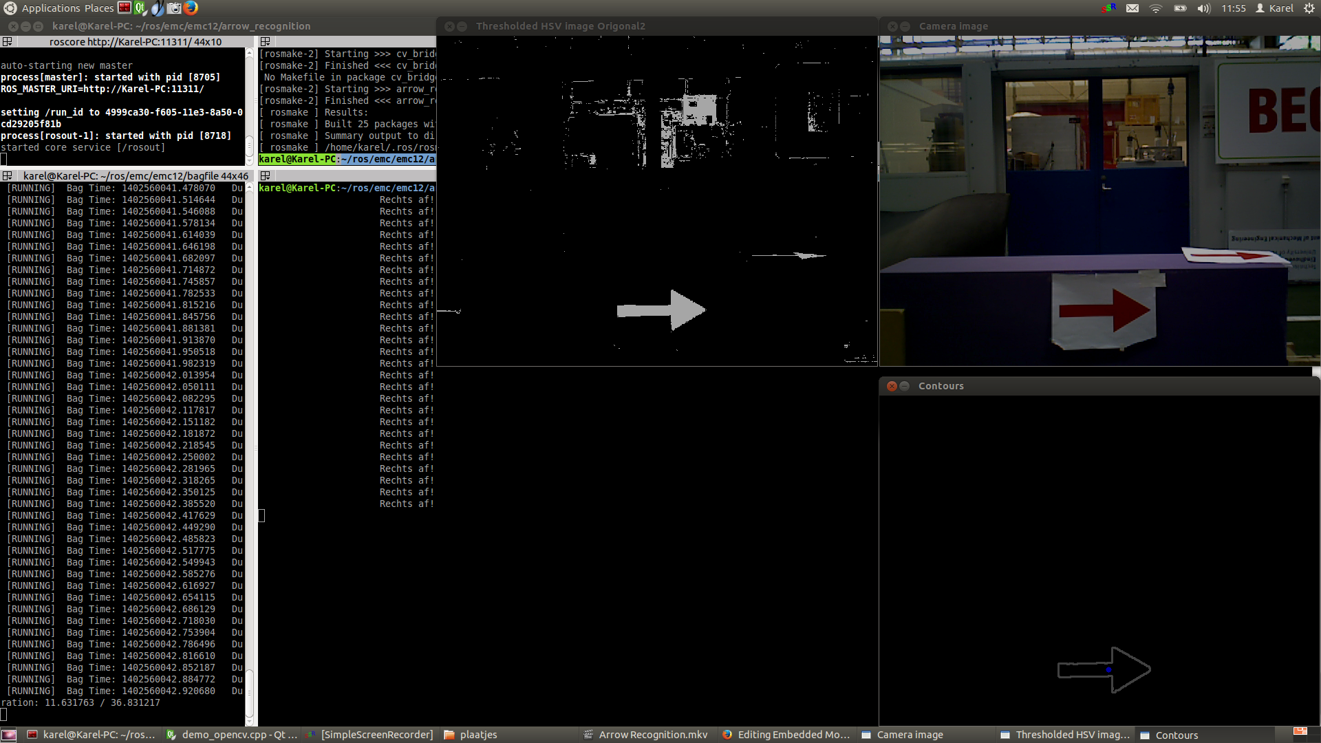
Arrow Recognition

For the recognition of arrows in the maze, a node calld arrow_recognition is created. The node is subscribed to the function imageCallback, for which the functioning will be described below. It sends messages (the direction of the arrow) over the channel /maze/arrow. Every 0.05 seconds the node spins and the imageCallback is performed, resulting into a message being sent over the defined channel. For image processing the OpenCV toolbox is used.

ROS RGB to OpenCV RGB

The first step is to convert the ROS RGB image (acquired by ROS subscription to /pico/asusxtion/rgb/image_color) to an OpenCV image so that it can be processed using this toolbox.

OpenCV RGB to HSV

The second step is to convert the RGB image to HSV color space (Hue, Saturation, Value), using cv::cvtColor. This technique allows tresholding of the image so certain specific HSV values can be extracted from the image. This will be done using the cv::inRange command, using a set of minimum and maximum values for Hue, Saturation and Value. These values are tuned iteratively by simulating pre-recorded bagfiles. Also, reference is taken from the picture and table below.

H = 180° (Cyan) H = 0° (Red) V \ S 1 ¾ ½ ¼ 0 ¼ ½ ¾ 1 1                   ⅞                   ¾                   ⅝                   ½                   ⅜                   ¼                   ⅛                   0	H = 210° (Blue-Cyan) H = 30° (Yellow-Red) V \ S 1 ¾ ½ ¼ 0 ¼ ½ ¾ 1 1                   ⅞                   ¾                   ⅝                   ½                   ⅜                   ¼                   ⅛                   0
H = 240° (Blue) H = 60° (Yellow) V \ S 1 ¾ ½ ¼ 0 ¼ ½ ¾ 1 1                   ⅞                   ¾                   ⅝                   ½                   ⅜                   ¼                   ⅛                   0	H = 270° (Magenta-Blue) H = 90° (Green-Yellow) V \ S 1 ¾ ½ ¼ 0 ¼ ½ ¾ 1 1                   ⅞                   ¾                   ⅝                   ½                   ⅜                   ¼                   ⅛                   0
H = 300° (Magenta) H = 120° (Green) V \ S 1 ¾ ½ ¼ 0 ¼ ½ ¾ 1 1                   ⅞                   ¾                   ⅝                   ½                   ⅜                   ¼                   ⅛                   0	H = 330° (Red-Magenta) H = 150° (Cyan-Green) V \ S 1 ¾ ½ ¼ 0 ¼ ½ ¾ 1 1                   ⅞                   ¾                   ⅝                   ½                   ⅜                   ¼                   ⅛                   0

Erode and Dilate Picture

The third step is to erode and dilate the acquired, HSV tresholded image. The function of eroding is that it computes a local minimum over the area of the kernel. A kernel is scanned over the image, the minimal pixel value overlapped by the kernel is computed and the original image will be replaced by the pixel under the anchor point with that minimal value. For dilation, the maximal value anchor point is used.[1]

Both functions together can be used to remove noise from the arrow and fill gaps inside the arrow up to ensure better edge detection. (Using cv::erode and cv:dilate.)

Blurring Image

Using cv::blur and cv:equalizeHist, the image is smoothed and the intensity range is stretched out. This results into an image for which the edges are easier to detect.

Canny Edge Detection

Now that several OpenCV functions have been used to modify the image, an edge detection function (cv::Canny) can be applied to extract a set of edges from the image. The function makes use of noise filtering, intensity gradients, suppression of pixels not belonging to the edge and hysteresis. [2]

Find Contours

Now that the edges have been detected succesfully, we can start creating closed contours from these edges, using cv::findContours to detect and cv:drawContours to draw the detected contours.

Select arrow contour using constraints

Now that all the contours have been found succesfully, we can try to select the arrow contour from the set of all contours identified. For this, a set of constraints is constructed, which will be discussed below.

• Looping over all the contours found, using cv:boundingRect, rectangles will be fitted over all the contours and the (x,y) position of all the corners of these rectangles will be logged. The first constraint can now be applied already: The length of the rectangle in x direction has to has to be bigger than 2.05 times the y direction and smaller than 2.35 times the y direction of the rectangle.

• Using cv::approxPolyDP we can approximate the areas of all the contours left, we will call this area a. The next step is to use cv:convexHull, which creates a convex hull around all the contours, we will call this area b. A nice property of the arrow we can use is the relation between a and b, which is always around 0.6. Furthermore we can only select contours that have b>3000 and a>2000.

• Ultimately, the only contour passing this set of constraints is the desired contour of the arrow.

Determine arrow direction using mass moments

Now that the arrow has been succesfully extracted from the image, we can start detecting the direction of the arrow. For this, the mass middle (x,y) will be detected using the cv:moments function. These coordinates will be compared with the middle of the bounded rectangle, created one step earlier. If the mass middle is more to the left than the middle of the bounded rectangle, we have found and arrow to the left! And vice versa for an arrow to the right, of course.

Memory

The created algorithm is now able to select the arrow contour and determine the direction. The last step is to define the message that has to be sent via the publisher, which is either a 1 (left arrow detected), a 0 (no arrow detected) or a -1 (right arrow detected). For robust selection, an exponential moving average is used. For this, a rolling average variable and two weighting factors \alpha and \beta are defined. If a direction is detected, this rolling average variable will be updated via a convex combination of the detected value and the memory of the rolling_avg variable.

rolling_avg = (alpha*detected_direction)+(1.0-alpha)*rolling_avg

where: detected_direction = 1 (if left) and detected_direction = -1 (if right)

When no direction is detected, the following formula is applied:

rolling_avg = (1.0-beta)*rolling_avg;

This will result into the exponential moving average to go towards 0.

Overview process

Below pictures are shown describing the entire process. There should be noted that probably the HSV values can be set stricter to select even less contours, although some room is given to ensure robustness for variations of the light level in the area PICO will drive.

Original image

HSV Treshold

Dilate

Erode

Blur

Canny

Final contour after applying constraints

Change log

09-05

Created scipt corridor_challenge.cpp with basic siteval to recognize conditions

13-05

• Testing corridor_challenge on Pico.

With new input from experiments: updated the corridor_challenge.cpp to corridor_challenge_v2.cpp. Brought the function sit-eval withing the callback loop for sensor messages. This way, the situation is evaluated and updated whenever new laser data is present. Some minor typo's. Added a situation that when things are to close (hard constraint) pico shuts down. After testing it was revealed that pico is stuck in condition 0 (does not know where he is).

15-05

• Revised corridor_challenge_v2.cpp -> renamed to corridorchallenge_v2.cpp and added some new functions:
• Extended laser 'vision' with left- and right diagonal view and updated amount of laser data used for each 'vision' vector.
• Extended the amount of possible situation PICO can be in to nine. Currently using:

- Corridor
- T-Junction (L+R)
- Crossing
- Corner (L+R)
- Dead End
- Exit

• Added a function that compares the left and right laser data and 'strafes' PICO to the middle using the y coordinate.
• Added an 'integrator'-like function that aligns the front vector of PICO to the walls of the corridor.
• Included front laser data to this function to ensure 'backup' when PICO comes too close to a wall.
• Added corresponding functions to new situations.
• Tweaked variables to ensure functioning simulations. (Allowance of some initial angle with reference to wall 'disturbance'). PICO is currently able to pass corridors, T-junctions and corners, for this however, the amount of possible situations PICO can be in is reduced for the sake of simplicity.

Final Design

The final design that was used was corridor_challenge_v2. It's goal was to use the laser data to recognize one of 9 conditions (ranging from freedom, corridor) and act in a preprogrammed way (outside of the loop) on how to handle these, and then turn on the loop again.

Result

Due to some unforeseen circumstances, corridorchallenge v3 failed to load on PICO. We resorted back to v2, which, while less robust, was still able to find the t-junction and act accordingly. The result was a first place in the "limited speed" category, with a time close to 20 seconds.

Maze Challenge

The goal of the Maze Challenge is to have PICO drive autonomously through a maze and successfully navigate itself towards the exit. There are three major assumptions

• (1) The Maze is two dimensional (all the walls, as well as the entrance and exits are on the ground floor level. There is no way to go either up or down).
• (2) Both the entrance and the exits are on the outer edge of the maze.
• (3) The maze does not change with time.

While these assumptions might seem redundant, they are of major importance when determining the strategy

Planning

Week 5

• Group meeting discussing the new strategy to finish solve the maze challenge
• Start coding on the line detection script

Week 6

• Debugging and finalizing the line detection script
• Beginning with coding the function for map generation
• Beginning with function to combine line detection with a situation evaluation

Week 7

• Lecture

Week 8

• Lecture

Software architecture / Road map

Line Detection

When regarding the designed software from the corridor competition, it became apparent that simply reading out the laser range data and comparing it against a set of reference values to determine the current situation was not really a robust solution. A better alternative would be to recognize lines surrounding PICO, instead of data points, and use this information to evaluate the situation.

(1) Line recognition of the upcoming junction, which is also robust against small gaps. The point where the two lines intersect is stored for later use. (2) Pico continous to drive until a second line (down the corridor) can be plotted. The point where the second line of the junction and the corridor meet is saved. The two saved points can now be used to estimate the corridor width. (3) Finally, with the width known, an arc is plotted around the corner of the corridor, allowing PICO to go around the corner. Because of the way the new trajectory is plotted, the corner may vary in width while PICO will still be able to end up in the middle of the corridor.

Strategy

Because of the three assumptions earlier, there are two practical ways to solve the maze.

• Always go right. Assuming that the error and the entrance is indeed on the edge of the maze, a simple right wall follower would always find the exit. However, there is no guarantee that all the possible routes are explored, and hence it is not possible to generate the shortest route.
• Take every possible corner. While this can be very time consuming, using clever algorithms (see [3]) it can be assured that the maze it thoroughly explored and that, at the end of the run, an entire map is available which could be used to find the shortest route to the exit.

Here, a trade-off has to be made. The first strategy is pretty easy to implement, and although it is not the fastest way, it is very robust. Because of this robustness, this strategy is implemented first to assure PICO fins an exit. Then, if time allows, the second strategy will be attempted.

Changelog

27 05

Created 3 line detection algorithms. First algorithm calculates the line between two subsequent points in r-theta space (Hough transform) and compares these values with the line between the next two points. If the next line is, within tolerances, similar to the first line, its point is added to the line and the next line is compared to the first line. To allow for gaps in the walls or incorrect measurements, a certain number of lines is allowed to be misaligned with the reference line if another line follows that does have the correct orientation. If this number of 'gap-lines' is exceeded, the algorithm returns to the first point that misaligned with the reference line and a new line is started from there. If the number of elements contained in the line is shorter than a certain value, the line is discarded as irrelevant. This algorithm proved unreliable and produced many interrupted lines.

In the second version the found lines are once more represented in r-theta coordinates and once again compared to each other in an attempt to sew interupted lines together. This proved not as effective as hoped.

A start was made with the third version, which functiosn similarly to the first version but compares lines between two points that are 10 measrements away. More accurately described in the update of 06 06.

06 06

After some investigation, it turned out that the measurement was relatively noisy, especially close to the robot. The third version is very similar to the first version, but uses two measurement points, a variable number of elements apart. This results in a low pass filtering of the laser data. The higher the number of elements, the smoother the line becomes, but the harder corners are to accurately detect. Another difficulty is that one line may now span acros an opening, such as a corridor, and in some cases it recognizes a diagonal line that does not exist. To prevent this, a constraint is added that does not allow the two points that are considered to be further apart than a certain threshold. This algorithm has a lot of parameters to tune, 6, but shows good results.

11 06

To be better able of coping with the uncertainty of the measurements and interpretation of the measurements by the line detection algorithm, a world model is added in three iterations.

The first iteration is a crude attempt, not using the line detection, but simply creating a discrete grid of Pico's surrounding and counting the number of measurements that fall within each grid point. After each measurement the previous measurement is partially forgotten. This works, but is memory consuming and inaccurate.

The second iteration is based on the first observation of Pico. If the line detection finds a line with similar orientation and that ends or starts within a certain tolerance of a line in the first observation of Pico, a number of points is added to that line. After each measurement, each line also loses a number of points and when the line has no points left, it is removed from the world model. If no match is found for a line within the world model, the new line is added to the world model. To compensate for the movement of Pico, all lines are moved a little if the robot moves forward, all lines are turned around if the robot turns in a dead end and if Pico takes a corner, it forgets the world model.

The third iteration also includes a section that updates the lines in the world model. If the starting or ending point of a measured line is close to the start or end point of a line in the world model, the location of that point is averaged between the two. If a measured line has a start or ending point that greatly exceeds the line in the world model, this point is used in the world model. This way, if a fractured line is present in the world model, the world model will be improved once the line is measured as a whole and the second fracture of the line will be forgotten over time.

12 06

Using the new way of representing the world around Pico, in lines with starting and ending coordinates, requires a new state machine to let Pico determine how to interpret the lines is observes.

To do this, four regions are specified: near right, far right, far left and near left. These regions have variable dimensions and locations with respect to the origin, Pico. The state machine searches for starting points in the left regions and ending points in the right regions to determine if an event could take place. If another starting or ending point is near by, the found point indicates a fracture in the world model and not a possible corner and the event is rejected. Using the information from these four regions, all nine possibly states of Pico can be determined, as described in the corridor challenge.

Experiments

22-05

• Found and tweaked the previously used script corridor_challenge_v2, based on new calculations. While it did work for one turn, a new calculations showed a situation where an error would occur when taking two turns successively. This turned out o also be true in practice, which again shows the importance of calculations and proper simulation.
• Experienced a new bug that would make PICO disconnect from the server for no apparent reason.
• Recorded a bag-file for line detection.

28-05

• Tested a new line detection script

Final Design

Final result

PICO succesfully found the exit